
PLEASE NOTE:
We are currently in the process of updating this chapter and we appreciate your patience whilst this is being completed.
Bias in Epidemiological Studies
While the results of an epidemiological study may reflect the true effect of an exposure(s) on the development of the outcome under investigation, it should always be considered that the findings may in fact be due to an alternative explanation1.
Such alternative explanations may be due to the effects of chance (random error), bias or confounding which may produce spurious results, leading us to conclude the existence of a valid statistical association when one does not exist or alternatively the absence of an association when one is truly present1.
Observational studies are particularly susceptible to the effects of chance, bias and confounding and these factors need to be considered at both the design and analysis stage of an epidemiological study so that their effects can be minimised.
Bias
Bias may be defined as any systematic error in an epidemiological study that results in an incorrect estimate of the true effect of an exposure on the outcome of interest.1
- Bias results from systematic errors in the research methodology.
- The effect of bias will be an estimate either above or below the true value, depending on the direction of the systematic error.
- The magnitude of bias is generally difficult to quantify, and limited scope exists for the adjustment of most forms of bias at the analysis stage. As a result, careful consideration and control of the ways in which bias may be introduced during the design and conduct of the study is essential in order to limit the effects on the validity of the study results.
Common types of bias in epidemiological studies
More than 50 types of bias have been identified in epidemiological studies, but for simplicity they can be broadly grouped into two categories: information bias and selection bias.
1. Information bias
Information bias results from systematic differences in the way data on exposure or outcome are obtained from the various study groups.1 This may mean that individuals are assigned to the wrong outcome category, leading to an incorrect estimate of the association between exposure and outcome.
Errors in measurement are also known as misclassifications, and the magnitude of the effect of bias depends on the type of misclassification that has occurred. There are two types of misclassification – differential and non-differential – and these are dealt with elsewhere (see “Sources of variation, its measurement and control”).
Observer bias may be a result of the investigator’s prior knowledge of the hypothesis under investigation or knowledge of an individual's exposure or disease status. Such information may influence the way information is collected, measured or interpretation by the investigator for each of the study groups.
For example, in a trial of a new medication to treat hypertension, if the investigator is aware which treatment arm participants were allocated to, this may influence their reading of blood pressure measurements. Observers may underestimate the blood pressure in those who have been treated, and overestimate it in those in the control group.
Interviewer bias occurs where an interviewer asks leading questions that may systematically influence the responses given by interviewees.
Minimising observer / interviewer bias:
- Where possible, observers should be blinded to the exposure and disease status of the individual
- Blind observers to the hypothesis under investigation.
- In a randomised controlled trial blind investigators and participants to treatment and control group (double-blinding).
- Development of a protocol for the collection, measurement and interpretation of information.
- Use of standardised questionnaires or calibrated instruments, such as sphygmomanometers.
- Training of interviewers.
Recall (or response) bias - In a case-control study data on exposure is collected retrospectively. The quality of the data is therefore determined to a large extent on the patient's ability to accurately recall past exposures. Recall bias may occur when the information provided on exposure differs between the cases and controls. For example an individual with the outcome under investigation (case) may report their exposure experience differently than an individual without the outcome (control) under investigation.
Recall bias may result in either an underestimate or overestimate of the association between exposure and outcome.
Methods to minimise recall bias include:
- Collecting exposure data from work or medical records.
- Blinding participants to the study hypothesis.
Social desirability bias occurs where respondents to surveys tend to answer in a manner they feel will be seen as favourable by others, for example by over-reporting positive behaviours or under-reporting undesirable ones. In reporting bias, individuals may selectively suppress or reveal information, for similar reasons (for example, around smoking history). Reporting bias can also refer to selective outcome reporting by study authors.
Performance bias refers to when study personnel or participants modify their behaviour / responses where they are aware of group allocations.
Detection bias occurs where the way in which outcome information is collected differs between groups. Instrument bias refers to where an inadequately calibrated measuring instrument systematically over/underestimates measurement. Blinding of outcome assessors and the use of standardised, calibrated instruments may reduce the risk of this.
2. Selection bias
Selection bias occurs when there is a systematic difference between either:
- Those who participate in the study and those who do not (affecting generalisability) or
- Those in the treatment arm of a study and those in the control group (affecting comparability between groups).
That is, there are differences in the characteristics between study groups, and those characteristics are related to either the exposure or outcome under investigation. Selection bias can occur for a number of reasons.
Sampling bias describes the scenario in which some individuals within a target population are more likely to be selected for inclusion than others. For example, if participants are asked to volunteer for a study, it is likely that those who volunteer will not be representative of the general population, threatening the generalisability of the study results. Volunteers tend to be more health conscious than the general population.
Allocation bias occurs in controlled trials when there is a systematic difference between participants in study groups (other than the intervention being studied). This can be avoided by randomisation.
Loss to follow-up is a particular problem associated with cohort studies. Bias may be introduced if the individuals lost to follow-up differ with respect to the exposure and outcome from those persons who remain in the study. The differential loss of participants from groups of a randomised control trial is known as attrition bias.
• Selection bias in case-control studies
Selection bias is a particular problem inherent in case-control studies, where it gives rise to non-comparability between cases and controls. In case-control studies, controls should be drawn from the same population as the cases, so they are representative of the population which produced the cases. Controls are used to provide an estimate of the exposure rate in the population. Therefore, selection bias may occur when those individuals selected as controls are unrepresentative of the population that produced the cases.
The potential for selection bias in case-control studies is a particular problem when cases and controls are recruited exclusively from hospital or clinics. Such controls may be preferable for logistic reasons. However, hospital patients tend to have different characteristics to the wider population, for example they may have higher levels of alcohol consumption or cigarette smoking. Their admission to hospital may even be related to their exposure status, so measurements of the exposure among controls may be different from that in the reference population. This may result in a biased estimate of the association between exposure and disease.
For example, in a case-control study exploring the effects of smoking on lung cancer, the strength of the association would be underestimated if the controls were patients with other conditions on the respiratory ward, because admission to hospital for other lung diseases may also be related to smoking status. More subtly, the effect of alcohol on liver disease could potentially be underestimated if controls are taken from other wards: higher than average alcohol consumption may result in admission for a variety of other conditions, such as trauma.
As the potential for selection bias is likely to be less of a problem in population-based case-control studies, neighbourhood controls may be a preferable choice when using cases from a hospital or clinic setting. Alternatively, the potential for selection bias may be minimised by selecting controls from more than one source. For example, the use of both hospital and neighbourhood controls.
• Selection bias in cohort studies
Selection bias can be less of problem in cohort studies compared with case-control studies, because exposed and unexposed individuals are enrolled before they develop the outcome of interest.
However, selection bias may be introduced when the completeness of follow-up or case ascertainment differs between exposure categories. For example, it may be easier to follow up exposed individuals who all work in the same factory, than unexposed controls selected from the community (loss to follow-up bias). This can be minimised by ensuring that a high level of follow-up is maintained among all study groups.
The healthy worker effect is a potential form of selection bias specific to occupational cohort studies. For example, an occupational cohort study might seek to compare disease rates amongst individuals from a particular occupational group with individuals in an external standard population. There is a risk of bias here because individuals who are employed generally have to be healthy in order to work. In contrast, the general population will also include those who are unfit to work. Therefore, mortality or morbidity rates in the occupation group cohort may be lower than in the population as a whole.
In order to minimise the potential for this form of bias, a comparison group should be selected from a group of workers with different jobs performed at different locations within a single facility1; for example, a group of non-exposed office workers. Alternatively, the comparison group may be selected from an external population of employed individuals.
• Selection bias in randomised trials
Randomised trials are theoretically less likely to be affected by selection bias, because individuals are randomly allocated to the groups being compared, and steps should be taken to minimise the ability of investigators or participants to influence this allocation process. However, refusals to participate in a study, or subsequent withdrawals, may affect the results if the reasons are related to both exposure and outcome.
Confounding
Confounding, interaction and effect modification
Confounding provides an alternative explanation for an association between an exposure (X) and an outcome. It occurs when an observed association is in fact distorted because the exposure is also correlated with another risk factor (Y). This risk factor Y is also associated with the outcome, but independently of the exposure under investigation, X. As a consequence, the estimated association is not that same as the true effect of exposure X on the outcome.
An unequal distribution of the additional risk factor, Y, between the study groups will result in confounding. The observed association may be due totally, or in part, to the effects of differences between the study groups rather than the exposure under investigation.1
A potential confounder is any factor that might have an effect on the risk of disease under study. This may include factors with a direct causal link to the disease, as well as factors that are proxy measures for other unknown causes, such as age and socioeconomic status.2
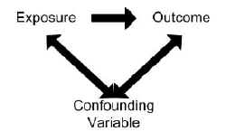
In order for a variable to be considered as a confounder:
- The variable must be independently associated with the outcome (i.e. be a risk factor).
- The variable must also be associated with the exposure under study in the source population.
- The variable should not lie on the causal pathway between exposure and disease.
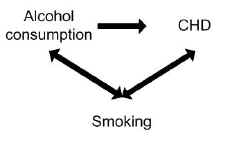
Examples of confounding
A study found alcohol consumption to be associated with the risk of coronary heart disease (CHD). However, smoking may have confounded the association between alcohol and CHD.
Smoking is a risk factor in its own right for CHD, so is independently associated with the outcome, and smoking is also associated with alcohol consumption because smokers tend to drink more than non-smokers.
Controlling for the potential confounding effect of smoking may in fact show no association between alcohol consumption and CHD.
Effects of confounding
Confounding factors, if not controlled for, cause bias in the estimate of the impact of the exposure being studied. The effects of confounding may result in:
- An observed association when no real association exists.
- No observed association when a true association does exist.
- An underestimate of the association (negative confounding).
- An overestimate of the association (positive confounding).
Controlling for confounding
Confounding can be addressed either at the study design stage, or adjusted for at the analysis stage providing sufficient relevant data have been collected. A number of methods can be applied to control for potential confounding factors and the aim of all of them is to make the groups as similar as possible with respect to the confounder(s).
Controlling for confounding at the design stage
Potential confounding factors may be identified at the design stage based on previous studies or because a link between the factor and outcome may be considered as biologically plausible. Methods to limit confounding at the design stage include randomisation, restriction and matching.
• Randomisation
This is the ideal method of controlling for confounding because all potential confounding variables, both known and unknown, should be equally distributed between the study groups. It involves the random allocation (e.g. using a table of random numbers) of individuals to study groups. However, this method can only be used in experimental clinical trials.
• Restriction
Restriction limits participation in the study to individuals who are similar in relation to the confounder. For example, if participation in a study is restricted to non-smokers only, any potential confounding effect of smoking will be eliminated. However, a disadvantage of restriction is that it may be difficult to generalise the results of the study to the wider population if the study group is homogenous.1
• Matching
Matching involves selecting controls so that the distribution of potential confounders (e.g. age or smoking status) is as similar as possible to that amongst the cases. In practice this is only utilised in case-control studies, but it can be done in two ways:
- Pair matching - selecting for each case one or more controls with similar characteristics (e.g. same age and smoking habits)
- Frequency matching - ensuring that as a group the cases have similar characteristics to the controls
Detecting and controlling for confounding at the analysis stage
The presence or magnitude of confounding in epidemiological studies is evaluated by observing the degree of discrepancy between the crude estimate (without controlling for confounding) and the adjusted estimate after accounting for the potential confounder(s). If the estimate has changed and there is little variation between the stratum specific ratios (see below), then there is evidence of confounding.
It is inappropriate to use statistical tests to assess the presence of confounding, but the following methods may be used to minimise its effect.
• Stratification
Stratification allows the association between exposure and outcome to be examined within different strata of the confounding variable, for example by age or sex. The strength of the association is initially measured separately within each stratum of the confounding variable. Assuming the stratum specific rates are relatively uniform, they may then be pooled to give a summary estimate as adjusted or controlled for the potential confounder. An example is the Mantel-Haenszel method. One drawback of this method is that the more the original sample is stratified, the smaller each stratum will become, and the power to detect associations is reduced.
• Multivariable analysis
Statistical modelling (e.g. multivariable regression analysis) is used to control for more than one confounder at the same time, and allows for the interpretation of the effect of each confounder individually. It is the most commonly used method for dealing with confounding at the analysis stage.
• Standardisation
Standardisation accounts for confounders (generally age and sex) by using a standard reference population to negate the effect of differences in the distribution of confounding factors between study populations. See “Numerators, denominators and populations at risk” for more details.
Residual confounding
It is only possible to control for confounders at the analysis stage if data on confounders were accurately collected. Residual confounding occurs when all confounders have not been adequately adjusted for, either because they have been inaccurately measured, or because they have not been measured (for example, unknown confounders). An example would be socioeconomic status, because it influences multiple health outcomes but is difficult to measure accurately.3
Interaction (effect modification)
Interaction occurs when the direction or magnitude of an association between two variables varies according to the level of a third variable (the effect modifier). For example, aspirin can be used to manage the symptoms of viral illnesses, such as influenza. However, whilst it may be effective in adults, aspirin use in children with viral illnesses is associated with liver dysfunction and brain damage (Reye’s syndrome).4 In this case, the effect of aspirin on managing viral illnesses is modified by age.
Where interaction exists, calculating an overall estimate of an association may be misleading. Unlike confounding, interaction is a biological phenomenon and should not be statistically adjusted for. A common method of dealing with interaction is to analyse and present the associations for each level of the third variable. In the example above, the odds of developing Reye’s syndrome following aspirin use in viral illnesses would be far greater in children compared to adults, and this would highlight the role of age as an effect modifier. Interaction can be confirmed statistically, for example using a chi-squared test to assess for heterogeneity in the stratum-specific estimates. However, such tests are known to have a low power for detecting interaction5 and a visual inspection of stratum-specific estimates is also recommended.
References
- Hennekens CH, Buring JE. Epidemiology in Medicine, Lippincott Williams & Wilkins, 1987.
- Carneiro I, Howard N. Introduction to Epidemiology. Open University Press, 2011.
- http://www.edmundjessop.org.uk/fulltext.doc - Accessed 20/02/16
- McGovern MC. Reye’s syndrome and aspirin: lest we forget. BMJ 2001;322:1591.
- Marshall SW. Power for tests of interaction: effect of raising the type 1 error rate. Epidemiological perspectives and innovations 2007;4:4.
© Helen Barratt, Maria Kirwan 2009, Saran Shantikumar 2018