
Health Economics: 7 - Decision Analysis
Decision analysis is now extensively used for economic evaluation modelling in health care (see, for example, Briggs, Sculpher and Claxton, 2006). It is used when the outcomes of an event are uncertain, but it is possible to assign a probability to each possible different outcome. For example, a drug may not cure every case that it is administered for, but is known to work in 80% of cases and has known side-effects in 5% of cases; or a surgical operation has been found to succeed in 75% of cases but has an operative mortality rate of 1%. Decision analysis is particularly valuable when decisions are not simply about a single choice between actions, but require strategies that incorporate multiple choices about different actions. For example, if a drug does not work then a second-line drug may be used, or if surgery does not work then drug therapy may be tried. Decision analysis is a way of structuring the different options so that the best strategy can be determined.
Decision analysis relies on the concept of expected values. The expected value of something can be thought of as its average value when it is repeated many times. For example, if a treatment produces a gain of 2 Quality Adjusted Life Years (QALYs) per person in 80% of cases and a gain of 1 QALY per person in the remaining 20%, then out of 100 patients the total gain will be (2x80) + (1x20) = 180. This means that the average gain is 1.8 QALYs per patient, which is the expected value. In reality, it is unlikely that the probabilities of 0.8 and 0.2 would produce exactly 80 and 20 in a population of 100, which is why the assumption of large numbers is made.
Generalising this, the expected value of an event is calculated as the sum over all possible outcomes of the probability of each outcome multiplied by its value. For example, if an activity X has two outcomes a and b which have probabilities P(a) and P(b) and values U(a) and U(b), the expected value of X is:
![]()
In economic appraisals in health care, decision analysis calculates the expected values of both costs and benefits and also ICERs, though the last of these is more complicated. They usually take the following form:
- Structure the problem by constructing a mathematical model of decision-making, usually a decision tree:
* Identify the decisions to be made between alternative actions and describe those alternatives
* List the possible outcomes of each alternative for each decision
* Specify the sequence of events that follow from each decision
- Assign probabilities to chance events.
- Assign values to all possible outcomes of chance events.
- Calculate the expected value of each possible strategy.
- Perform sensitivity analyses by systematically changing the assumptions in (1) - (3) to see the impact on the result of (4).
This will be explained using a decision tree first presented by Morris, Devlin, Parkin and Spencer (2012). A decision tree uses a diagrammatic illustration of a decision problem. Nodes, representing key elements of the decision problem are connected by lines, called paths, representing links between them. The paths run from left to right and imply a sequence in that order. Decisions that are controlled by a decision maker are called decision nodes, conventionally drawn as squares:
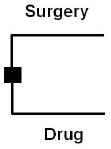
This shows that the decision is between surgery and drug therapy. The paths running from this are the consequences of choosing a particular alternative. It is possible to have more than two alternatives, but they must all be mutually exclusive.
Any chance occurrences that are not controlled by the decision-maker are called chance nodes or probability nodes, conventionally drawn as circles:
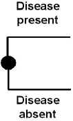
In this case, disease may be present or absent. The important aspect of this is that each of the alternatives must have a probability attached to it - in this case the probability that a disease is present or absent. There can be more than one outcome, but they must also be mutually exclusive and moreover they must be collectively exhaustive; that is, the sum of their probabilities must exactly equal one.
The final outcome associated with a path is a terminal node, conventionally drawn as a triangle:
![]()
Every path that does not lead to a chance event or decision must have a terminal node. In this case, the final outcome of a set of decisions and chance events is that the patient is cured.
A full decision tree would contain all of the relevant nodes and the paths between them. To this would be added the probabilities assigned to chance events and the values attached to each potential final outcome. It might look like this:
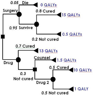
In this case, the initial choice of surgery leads to a chance node associated with surgery, where the possibility of operative mortality is included. Assuming that the patient survives, a further chance node represents the probability that they will be cured, leading to the final outcomes of being cured by surgery and not cured despite surgery. The initial choice of drug therapy leads to a node depicting the chance that the patient is cured or not. Being cured is a final outcome and leads to a terminal node. If the patient is not cured, a second decision is taken, to offer counselling, which again leads to a final outcome, or a second line drug, which again has a cured/not cured chance node, although this time both lead to final outcomes.
The expected value of the different options can then be calculated in stages, working from right to left. The expected value to a patient who survives surgery is (0.8*15) + (0.2*0.5) = 12.1 QALYs. This value is used to calculate the expected value of surgery for all patients, whether they survive or not, which is (0.05*0) + (0.95*12.1) = 11.495 QALYs.
The expected value of using Drug 2 is (0.5*10) + (0.5*1) = 5.5 QALYs. Since this is greater than the value of counselling, the decision following a failure of Drug 1 should be to try Drug 2, so the expected value of Drug 2 therapy is used in the calculation of the expected value of Drug 1, which is (0.7*13) + (0.3*5.5) = 10.75.
Surgery therefore produces, on average, a greater QALY gain, and the incremental benefit of surgery is (11.495 - 10.75) = 0.745 QALYs. Of course, in an economic evaluation, it would also be necessary to measure the costs of each terminal node and to calculate the expected value of costs for each decision option.
Other refinements are possible to this basic framework, of which the most important is a Markov Model, which may replace some or all of the chance nodes. Ordinary chance nodes imply a fixed sequence that has no time dimension, but that may not be realistic, particularly where this is intended to represent disease and therapeutic processes that are dynamic. For example, patients are not usually simply cured or not because of treatment, they may initially get worse, then improve, perhaps relapse and die, or if they do not they may improve again and may remain in that state until they die of something else, or improve further so that they can be thought of as cured.
Using the same example of a disease process for illustration, a Markov model will assume that each patient is at any time in one of a specific number of health states, called Markov states. During a specific time period, called a cycle, the patient may remain in the same state or move to one of the others, with a given probability of moving known as a transition probability. For example, suppose that there are three possible states - ‘well’, ‘sick’ and ‘dead’. The initial distribution of patients between these states is that they are all in the state ‘sick’. During the first cycle, some will become well, some will die and others will remain sick, giving a new distribution of states. This will be repeated during the second cycle for those who remain sick after the first cycle, but there will now also be patients who became well during the first cycle; they also may remain well, become sick or even die. However, those who died during the first cycle cannot of course move from that state and remain in it for all subsequent cycles. Such a state is called an absorbing state.
The cycles can be repeated as many times as required. The results of this will be a different distribution of health states over the population at each period. It is possible then to attach to each health state costs and benefits, for example the cost of being in each health state and the quality of life in it, and to calculate the sum over time of these. The impact of therapy may be to alter the probabilities, or the length of cycles, or both and it will be possible to calculate the sums of costs and benefits with and without therapy for use in an economic evaluation.
The length of the cycles and the number of times that they are repeated will be determined by the nature of the disease and the therapy. For example, a rapidly-changing acute illness might be modelled using short cycles over a short time period, whereas a slowly-developing chronic condition might be modelled by relatively long cycles over a long time.
© David Parkin 2017