
Introduction
Learning objectives: You will learn about standard error of a mean, standard error of a proportion, reference ranges, and confidence intervals. The earlier sections covered estimation of statistics. This section considers how precise these estimates may be. Please now read the resource text below.
Resource text
Standard error of the mean
A series of samples drawn from one population will not be identical. They will show chance variations from one to another, and the variation may be slight or considerable. For example, a series of samples of the body temperature of healthy people would show very little variation from one to another, but the variation between samples of the systolic blood pressure would be considerable. Thus the variation between samples depends partly on the amount of variation in the population from which they are drawn. Furthermore, it is a matter of common observation that a small sample is a much less certain guide to the population from which it was drawn than a large sample. In other words, the more people that are included in a sample, the greater chance that the sample will accurately represent the population, provided that a random process is used to construct the sample. A consequence of this is that if two or more samples are drawn from a population, then the larger they are, the more likely they are to resemble each other - again, provided that the random sampling technique is followed. Thus the variation between samples depends partly also on the size of the sample. If we draw a series of samples and calculate the mean of the observations in each, we have a series of means.
These means generally follow a normal distribution, and they often do so even if the observations from which they were obtained do not. This can be proven mathematically and is known as the "Central Limit Theorem". The series of means, like the series of observations in each sample, has a standard deviation. The standard error of the mean of one sample is an estimate of the standard deviation that would be obtained from the means of a large number of samples drawn from that population.
As noted above, if random samples are drawn from a population, their means will vary from one to another. The variation depends on the variation of the population and the size of the sample. We do not know the variation in the population so we use the variation in the sample as an estimate of it. This is expressed in the standard deviation. If we now divide the standard deviation by the square root of the number of observations in the sample we have an estimate of the standard error of the mean. It is important to realise that we do not have to take repeated samples in order to estimate the standard error; there is sufficient information within a single sample. However, the concept is that if we were to take repeated random samples from the population, this is how we would expect the mean to vary, purely by chance.
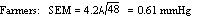
Example 1 A general practitioner has been investigating whether the diastolic blood pressure of men aged 20-44 differs between printers and farm workers. For this purpose, she has obtained a random sample of 72 printers and 48 farm workers and calculated the mean and standard deviations, as shown in table 1. Table 1: Mean diastolic blood pressures of printers and farmers
| Number | Mean diastolic blood pressure (mmHg) | Standard deviation (mmHg) | |
| Printers | 72 | 88 | 4.5 |
| Farmers | 48 | 79 | 4.2 |
To calculate the standard errors of the two mean blood pressures, the standard deviation of each sample is divided by the square root of the number of the observations in the sample. 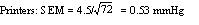
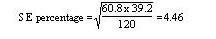
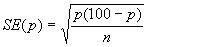
 These standard errors may be used to study the significance of the difference between the two means. Standard error of a proportion or a percentage Just as we can calculate a standard error associated with a mean so we can also calculate a standard error associated with a percentage or a proportion. Here the size of the sample will affect the size of the standard error but the amount of variation is determined by the value of the percentage or proportion in the population itself, and so we do not need an estimate of the standard deviation. Example 2 A senior surgical registrar in a large hospital is investigating acute appendicitis in people aged 65 and over. As a preliminary study he examines the hospital case notes over the previous 10 years and finds that of 120 patients in this age group with a diagnosis confirmed at operation, 73 (60.8%) were women and 47 (39.2%) were men. If p represents one percentage, 100-p represents the other. Then the standard error of each of these percentages is obtained by (1) multiplying them together, (2) dividing the product by the number in the sample, and (3) taking the square root:
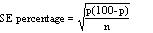
which for the appendicitis data given above is as follows:
Reference ranges
Swinscow and Campbell (2002) describe 140 children who had a mean urinary lead concentration of 2.18 mmol /24h, with standard deviation 0.87. The points that include 95% of the observations are 2.18 (1.96 x 0.87), giving an interval of 0.48 to 3.89. One of the children had a urinary lead concentration of just over 4.0 mmol /24h. This observation is greater than 3.89 and so falls in the 5% of observations beyond the 95% probability limits. We can say that the probability of each of these observations occurring is 5%. Another way of looking at this is to see that if you chose one child at random out of the 140, the chance that the child's urinary lead concentration will exceed 3.89, or is less than 0.48, is 5%. This probability is usually used expressed as a fraction of 1 rather than of 100, and written as p<0.05. Standard deviations thus set limits about which probability statements can be made. Some of these are set out in table 2. Table 2: Probabilities of multiples of standard deviation for a normal distribution
| Number of standard deviations (z) | Probability of getting an observation at least as far from the mean (two sided P) |
| 0 | 1.00 |
| 0.5 | 0.62 |
| 1.0 | 0.31 |
| 1.5 | 0.13 |
| 2.0 | 0.045 |
| 2.5 | 0.012 |
| 3.0 | 0.0027 |
To estimate the probability of finding an observed value, say a urinary lead concentration of 4.8 mmol /24h, in sampling from the same population of observations as the 140 children provided, we proceed as follows. The distance of the new observation from the mean is 4.8 - 2.18 = 2.62. How many standard deviations does this represent? Dividing the difference by the standard deviation gives 2.62/0.87 = 3.01. Table 2 shows that the probability is very close to 0.0027. This probability is small, so the observation probably did not come from the same population as the 140 other children. To take another example, the mean diastolic blood pressure of printers was found to be 88 mmHg and the standard deviation 4.5 mmHg. One of the printers had a diastolic blood pressure of 100 mmHg. The mean plus or minus 1.96 times its standard deviation gives the following two figures:

We can say therefore that only 1 in 20 (or 5%) of printers in the population from which the sample is drawn would be expected to have a diastolic blood pressure below 79 or above about 97 mmHg. These are the 95% limits. The 99.73% limits lie three standard deviations below and three above the mean. The blood pressure of 100 mmHg noted in one printer thus lies beyond the 95% limit of 97 but within the 99.73% limit of 101.5 (= 88 + (3 x 4.5)). The 95% limits are often referred to as a "reference range". For many biological variables, they define what is regarded as the normal (meaning standard or typical) range. Anything outside the range is regarded as abnormal. Given a sample of disease free subjects, an alternative method of defining a normal range would be simply to define points that exclude 2.5% of subjects at the top end and 2.5% of subjects at the lower end. This would give an empirical normal range . Thus in the 140 children we might choose to exclude the three highest and three lowest values. However, it is much more efficient to use the mean +/- 2SD, unless the dataset is quite large (say >400).
Confidence intervals
The means and their standard errors can be treated in a similar fashion. If a series of samples are drawn and the mean of each calculated, 95% of the means would be expected to fall within the range of two standard errors above and two below the mean of these means. This common mean would be expected to lie very close to the mean of the population. So the standard error of a mean provides a statement of probability about the difference between the mean of the population and the mean of the sample. In our sample of 72 printers, the standard error of the mean was 0.53 mmHg. The sample mean plus or minus 1.96 times its standard error gives the following two figures:

This is called the 95% confidence interval , and we can say that there is only a 5% chance that the range 86.96 to 89.04 mmHg excludes the mean of the population. If we take the mean plus or minus three times its standard error, the interval would be 86.41 to 89.59. This is the 99.73% confidence interval, and the chance of this interval excluding the population mean is 1 in 370. Confidence intervals provide the key to a useful device for arguing from a sample back to the population from which it came. With small samples - say under 30 observations - larger multiples of the standard error are needed to set confidence limits. These come from a distribution known as the t distribution, for which the reader is referred to Swinscow and Campbell (2002). Confidence interval for a proportion In a survey of 120 people operated on for appendicitis 37 were men. The standard error for the percentage of male patients with appendicitis is given by:
In this case this is 0.0446 or 4.46%. This is also the standard error of the percentage of female patients with appendicitis, since the formula remains the same if p is replaced by 100-p. With this standard error we can get 95% confidence intervals on the two percentages:

These confidence intervals exclude 50%. We can conclude that males are more likely to get appendicitis than females. This formula is only approximate, and works best if n is large and p between 0.1 and 0.9. A better method would be to use a chi-squared test, which is to be discussed in a later module. There is much confusion over the interpretation of the probability attached to confidence intervals. To understand it, we have to resort to the concept of repeated sampling. Imagine taking repeated samples of the same size from the same population. For each sample, calculate a 95% confidence interval. Since the samples are different, so are the confidence intervals. We know that 95% of these intervals will include the population parameter. However, without any additional information we cannot say which ones. Thus with only one sample, and no other information about the population parameter, we can say there is a 95% chance of including the parameter in our interval. Note that this does not mean that we would expect, with 95% probability, that the mean from another sample is in this interval.
Video 1: A video summarising confidence intervals. (This video footage is taken from an external site. The content is optional and not necessary to answer the questions.)
References
- Altman DG, Bland JM. BMJ 2005, Statistics Note Standard deviations and standard errors. Swinscow TDV, and Campbell MJ. BMJ Books 2009, Statistics at Square One, 10 th ed. Chapter 4.
Related links
- http://bmj.bmjjournals.com/cgi/content/full/331/7521/903