
Introduction
Learning Objectives: You will learn methods of summarising a single quantitative variable. This section covers means, medians, inter-quartile range, range, and standard deviations. Please now read the resource text below.
Resource text
Measures of Location
Mean or average The mean or average of n observations (pronounced x bar) is simply the sum of the observations divided by their number. Thus:
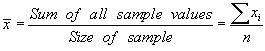
In equation 1, xi represents the individual sample values and Sxi their sum. The Greek letter 'S' (sigma) is the Greek capital 'S' and stands for sum. The median is the value at which half the observations are less than it and half are greater. The median is defined as the middle point of the ordered data. The calculation is described below.
Example 1: Calculation of mean and median Consider the following 5 birth weights in kilograms, recorded to 1 decimal place only: 1.2, 1.3, 1.4, 1.5, 2.1 The mean is defined as the sum of the observations divided by the number of observations. Thus mean = (1.2 + 1.3 + ... + 2.1)/5 = 1.50 kg. It is usual to quote one more decimal place for the mean than the data recorded. There are 5 observations, which is an odd number, so the median is the middle one of the observations. It is the (n + 1)/2 th in order of increasing size. In this case the median is the 3rd highest number which is 1.4 kg. If the number of observations was even, then the median is defined as the average of the n/2th and the n/2 + 1th. Thus if we had observed an additional value of 3.5 kg in the birth weight the median would be the average of the 3rd and the 4th observation in the ranking, namely the average of 1.4 and 1.5, which is 1.45 kg. The major advantage of the mean is that it uses all the data values, and is efficient, in a statistical sense. The main disadvantage of the mean is that it is vulnerable to what are known as outliers. Outliers are single observations which, if excluded from the calculations, have noticeable influence on the results. For example, if we had entered '21' instead of '2.1' in the calculation of the mean in example 1, we would find the mean changed from 1.50 kg to 7.98 kg. It does not necessarily follow, however, that outliers should be excluded from the final data summary or that they result from an erroneous measurement.
Median The median has the advantage that it is not affected by outliers, so for example the median in the example would be unaffected by replacing '2.1' with '21'. However, it is not statistically efficient, as it does not make use of all the individual data values.
Mode
A third measure of location, after the mean and median, is termed the mode. This is the value that occurs most frequently, or if the data are grouped, the grouping with the highest frequency. It is not used much in statistical analysis, since its value depends on the accuracy with which the data are measured, although it may be useful to describe the most frequent category for categorical data. The expression 'bimodal' distribution is used to describe a distribution with two peaks in it. This can be caused by mixing populations. For example, height might appear bimodal if one had men and women in the population. Some illnesses may raise a biochemical measure, so in a population containing healthy and ill people one might expect a bimodal distribution. However, some illnesses are defined by the measure, e.g. obesity or high blood pressure, and in this case the distributions are usually unimodal.
Video 1: A video summary of the mode, median and mean. (This video footage is taken from an external site. The content is optional and not necessary to answer the questions.)
Measures of Dispersion or Variability
Range and interquartile range
The range is given as the smallest and largest observation. This is the simplest measure of variability. Note that in statistics, unlike physics, a range is given by two numbers, not the difference between the smallest and largest. For some data, it is very useful because you would want to know these numbers, for example in a sample looking for the age of the youngest and oldest participants. If outliers are present, the range may give a distorted impression of the variability of the data, since all but two of the data points are not included in the estimate.
Quartiles
The quartiles, namely the lower quartile, the median (the second quartile), and the upper quartile, divide the data into four equal parts; that is, there will be approximately equal numbers of observations in the four sections - and exactly equal if the sample size is divisible by four and the measures are all distinct. The quartiles are calculated in a similar way to the median; first, order the data and then count the appropriate number from the bottom as shown in example 2. The interquartile range is a useful measure of variability and is derived from the lower and upper quartiles. The interquartile range is not vulnerable to outliers, and whatever the distribution of the data, we know that 50% of them lie within the interquartile range.
Example 2: Calculation of the quartiles
Suppose we had 18 birth weights arranged in increasing order.
1.51, 1.53, 1.55, 1.55, 1.79, 1.81, 2.10, 2.15, 2.18,
2.22, 2.35, 2.37, 2.40, 2.40, 2.45, 2.78, 2.81, 2.85.
The median is the average of the 9th and 10th observations (2.18+2.22)/2 = 2.20 kg. The first half of the data has 9 observations, so the first quartile is the 5th, namely 1.79 kg. Similarly, the 3rd quartile would be the 14th observation, namely 2.40 kg.
Standard deviation and variance
The standard deviation is calculated as follows:
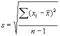
The expression is interpreted as: from each x value subtract the mean, square this difference, then add each of the n squared differences. This sum is then divided by (n - 1). This expression is known as the variance. The variance is expressed in square units, so we take the square root to return to the original units, which gives the standard deviation, s. Examining this expression it can be seen that if all the x's were the same they would be equal and so s would be zero. If the x's were widely scattered about, then s would be large. In this way, s reflects the variability in the data. The calculation of the standard deviation is described in example 3. The standard deviation is vulnerable to outliers, so if the 2.1 was replaced by 21 in example 3, we would get a very different result.
Example 3: Calculation of the standard deviation
Consider the data from example 1. The calculations are given in the following table. We found the mean to be 1.5 kg. We subtract this from each of the observations. Note the mean of this column is zero. This will always be the case: the positive deviations from the mean cancel the negative ones. A convenient method of removing the negative signs is by squaring the deviations, which is given in the next column to get 0.50 kgs2.
We need to find the average squared deviation. Common sense would suggest dividing by n, but it turns out that this gives an estimate of the population variance that is too small. This is because we are using the estimated mean in the calculation and we should really be using the true population mean. It can be shown that it is better to divide by the degrees of freedom, which is n minus the number of estimated parameters, in this case n-1. An intuitive way of looking at this is to suppose there were n telephone poles each 100 meters apart. How much wire would you need to link them? As with variation, here we are not interested in where the telegraph poles are, but simply how far apart they are. A moments thought should convince that we need n-1 lengths of 100 meter wire.
Calculation of the standard deviation
n = 5, Variance = 0.50/(5-1) = 0.125 kgs2, Standard deviation = sqrt(0.125) = 0.35 kg.
Why is the standard deviation useful?
It turns out in many situations that about 95% of observations will be within two standard deviations of the mean, known as a reference interval. It is this characteristic of the standard deviation which makes it so useful. It holds for a large number of measurements commonly made in medicine. In particular it holds for data that follow a normal distribution. Standard deviation is often abbreviated to SD in the medical literature. It will be denoted here, however, as SD(x), where the bracketed x is emphasised for a reason to be introduced later.
Video 2: A video summary of quantitative data. (This video footage is taken from an external site. The content is optional and not necessary to answer the questions.)
Reference
- Campbell MJ and Swinscow TDV. Blackwell 2009. Statistics at Square One 11th Ed Oxford