Health Economics: 5 - Techniques of Economic Appraisal

5.1 What is economic appraisal?

Economic appraisal and economic evaluation are general names for a set of techniques that weigh up the costs of an action against the benefits that it provides. The distinction between appraisal and evaluation is that appraisal is undertaken
before the action is taken, to decide what is to be done, and evaluation is undertaken after the action, to monitor its effects. However, except in certain circumstances this distinction is usually forgotten and the terms are used interchangeably in
much of health economics. In recent years, the expression ‘evaluation’ has become dominant in the health economics literature, but ‘appraisal’ is used here.

The usual label given to this activity in economics is cost-benefit analysis (CBA). However, that term is often reserved in health economics for a particular technique related to the measurement of overall allocative efficiency, as defined in Section
1.4.1. This will be explained below. CBA is a structured approach to help decision makers choose between alternative ways of using resources. Its main aim is to measure efficiency in areas where there is public involvement and there are therefore
no market-based measures available to judge issues of efficiency. Equity issues should, in principle, be considered as part of an economic appraisal, but there are fewer formal techniques available to analyse this aspect.

5.2 Formulating an appraisal

One way to look at how an appraisal is carried out is to consider it as a process with stages, as follows:

The problem is always the starting point of an appraisal. This may seem obvious, but in fact it is often solutions that are, wrongly, regarded as the starting point. From an appraisal point of view, the problem is not whether a
particular drug is cost-effective, but what is the most cost-effective way to deal with the problem that the new drug is licensed for. This may have an impact on the second stage, defining alternatives, which means different ways of dealing with the
problem. It is important to select the most relevant alternative, whatever it is – for example, another drug, another type of therapy, routine care without specific therapy or ‘do nothing’.

Enumeration of costs and benefits means the drawing up of a descriptive list of the costs and benefits that are to be included in the appraisal. Measurement means obtaining data to describe the levels of costs and benefits for the different
alternatives. Valuation is required to convert the data into values. For example, data on resource use should be converted into costs by applying to those data the value of the resources. Further details of how this is done in practice are given in
sections 5.4 and 5.5.

Calculation means combining the data on costs and benefits into the results that will be presented. The exact nature of this will depend on the type of appraisal that is carried out – see section 5.3 – and how uncertainty over the results is
dealt with – see section 5.6.

The endpoint is when a decision is taken on the basis of the appraisal. This will not be taken by an appraiser, but by someone who has the responsibility to make a decision. However, appraisers often do recommend a decision which is based on their
own appraisal, or imply such a recommendation. This is legitimate if the relevant decision rules are known. For example, there might be an accepted decision rule that states that if the benefits of a health intervention exceed its cost then it
should be provided to the population. A finding, for a particular intervention, that its benefits did exceed its costs may then lead to a recommendation that it should be provided.

One important factor in this is that an appraisal should be formulated and carried out with full awareness of which viewpoint is being taken. This arises because different actors in the health system – patients, health professionals and
government for example – may have different interests and concerns, so that what is efficient from one point of view may not be from another. This is important because it determines which type of appraisal is to be used, what constitutes a benefit
and a cost and how these are to be valued. Most appraisals will take the viewpoint of the health service, since that embodies most of those who have the legitimacy to decide which health care is to be provided. However, they may also take the
viewpoint of society as a whole, since that defines the recipients of health care as well as the ultimate funders of it. Whatever viewpoint is adopted, researchers should be explicit about which it is.

5.3 Types of economic appraisal

Although there are several different types of economic appraisal, we will concentrate here on those most likely to be encountered in health care. Unfortunately, there are different ways in which these types can be classified. This leads to
occasional disputes about how results of a particular type of appraisal should be interpreted or used. One way is to classify them according to what kind of efficiency they analyse. A second way is to classify them according to which costs and
benefits are measured and how this is done. A third way is to classify them according to the type of decision that they apply to. Although we will discuss all three types here, the most widespread and popular classification in health economics is
given by Drummond et al (2005), which uses both the measurement and decision type principles.

In what follows, we refer to what is being appraised as ‘alternatives’, reflecting the use of economic appraisal in health care in decision making about alternative ways of using health care resources. This includes many kinds of decisions,
including different ways of delivering health care, different types of health care and different treatment options.

5.3.1 Cost-benefit analysis (CBA)

In economics more generally, Cost-benefit analysis (CBA) starts with an inventory of all of the costs and benefits of each of the alternatives, whatever they are and whoever incurs them. This can be regarded as a balance sheet in which costs and
benefits are weighed up against each other.

However, in health economics CBA is usually defined, following Drummond et al, as a technique in which all costs and benefits are measured in terms of money. The rationale for this is that it is only possible to weigh up all of the costs
and benefits if they are measured in the same unit. Although in principle any common unit could be used, in practice money is the obvious and natural choice, as it is the measure of value most used in modern economies. The result of such a CBA would
be to establish which of the alternatives has the greatest net benefit – the difference between benefits and costs, which could of course be negative.

The main decision rule for CBA is that an activity should be undertaken if the sum of the benefits is greater than the sum of the costs or, identically, if the net benefit is positive. If only one activity with a positive net benefit can be
undertaken (because, for example, there are limited funds), then the rule is to choose the activity with the highest net benefit.

There is a theoretical basis for CBA in economics. If all of the costs and benefits are measured in the correct way – for example, all costs measure their true opportunity costs – and an alternative has a net benefit, it will lead to a Pareto
improvement. The way that this has been interpreted by Drummond et al is that CBA is therefore appropriate for answering questions about whether or not a health care programme should be implemented or a treatment should be used, rather than
which of a number of alternative programmes or interventions is the most efficient.

5.3.2 Option Appraisal

Option appraisal is a term used by the UK Treasury in the guidance that it gives to public bodies about how they should appraise and evaluate projects that are to be paid for from public funds, contained in its ‘Green Book’ (http://greenbook.treasury.gov.uk/);
the distinction between appraisal and evaluation is carefully kept to in this case. Option appraisal is a process in which different options for meeting an objective, defined by the aim of meeting some public need, are generated; CBA is applied to
these options; and the best solution for meeting the aims is chosen on the basis of the results. For example, an appraisal of a project for building a new acute hospital would not start as a comparison of the new hospital with existing facilities. It
would start with the need to provide acute services, generate different options for dealing with that need, which might include a new hospital build, examine the costs and benefits of each alternative and from this derive the economic case for the
new building, if it was found to be the best alternative. The economic case for the project would simply be part of a more general project appraisal included affordability and achievability and various types of impact assessment including on health,
the environmental and health and safety.

5.3.3 Cost-consequences analysis (CCA)

Cost-consequences analysis (CCA) is a form of CBA which does not try to put all of the costs and benefits into the same units. In particular, it accepts that there are different types of benefits that cannot be measured in the same units. This
distinguishes it from cost-effectiveness analysis, which is discussed below. The assumption is that in making decisions based on a CCA, different decision makers will place their own weights on the different benefits and on costs, implicitly if not
explicitly. CCA is of particular interest in public health because the National Institute for Health and Clinical Excellence (NICE) in England permits the use of CCA for public health interventions, unlike other health care. CCA is often referred to
as a disaggregated approach, because the benefits and costs are not combined into a single indicator such as net benefit or a cost-effectiveness ratio, which is defined below.

5.3.4 Cost-effectiveness Analysis (CEA)

Cost-effectiveness derives from the analysis of economic efficiency, where one alternative is preferred to another if it provides greater benefit at the same or lower cost, or lower cost for the same or greater benefit. This definition leaves open
the question of which of two alternatives is more efficient if one provides greater benefit than the other, but at a lower cost. However, under certain conditions – for example, that the alternatives can be reduced or increased in size to produce
any level of total cost or benefit – such comparisons can be made. A cost-effectiveness ratio (CER), defined as costs divided by benefits, can be calculated in order to do this. The CER most often used in health economics is called an incremental
CER, or ICER, where the costs and benefits of each alternative are calculated compared with their next best alternative, rather than with a common alternative.

The measurement principle for CEA is that costs are measured in terms of money, but that benefits are measured in units other than money. However, unlike CCA, all of the benefits are measured in the same units, usually because only one type of
benefit is considered. The obvious consequence of this is that costs and benefits are not weighed against each other. The ICER simply shows the cost of obtaining a unit of benefit. Whether that cost is worth incurring is a different question. So,
unlike CBA, which tells us whether or not health programmes or treatment are an efficient use of resources, CEA tells us which of the possible ways of providing those is the most efficient.

Drummond et al restrict the use of the term CEA in two ways. First, they regard CEA as being applicable only when both the costs and benefits of the alternatives differ from each other. The case where benefits are the same but costs differ
is called cost-minimisation analysis (CMA). However, this term is rarely used to describe analyses that have been carried out, although such analyses may well be quite widespread. Secondly, they restrict the measurement of benefits to be in ‘natural’
units, such as numbers of cases detected, changes in clinical measures like blood pressure or changes in undesirable biological markers. This is by contrast to the measurement of benefits in terms of changes in health-related quality of life, which
is given the different label of cost-utility analysis (CUA). This is discussed below.

The first decision rule for this kind of CEA is that we should reject any alternatives that are dominated by another alternative or combination of alternatives. This is economic efficiency in the strict sense described above, where the
dominated alternative has a greater cost with no greater benefits or lower benefits with no smaller costs. The choice between non-dominated alternatives is more complex. Where only one alternative can be chosen, that with the lowest ICER should be
chosen, but only if it is below a ceiling ratio, which is a level of the ICER which any alternative must meet if it is to be regarded as cost-effective. Where combinations of more than one alternative can be used, it is in principle necessary
to calculate the ICERS for every possible combination to decide which is most efficient and if any meet the ceiling ratio requirement.

These issues are often illustrated using a cost-effectiveness plane diagram (Black, 1990). ICERs are presented graphically as a combination of the costs and the effects of a health intervention, described in the diagram below as a ‘treatment’,
compared to some alternative. Costs are conventionally placed on the north-south axis and effects on the east-west axis. In both cases, these effects can be negative, zero or positive:

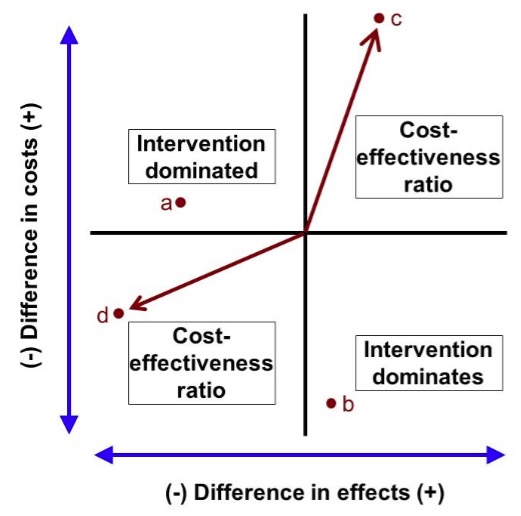
An intervention can be placed anywhere on this diagram according to its incremental costs and benefits. If it lies in the north-west quadrant, such as point A, the costs of the intervention are higher than the alternative, and its benefits are
lower. It is therefore unambiguously worse, and is said to be dominated by the alternative. Similarly, in the south-east quadrant, at a point such as B, costs are lower and benefits are higher, so the treatment dominates its alternative. In the
north-east quadrant, at a point such as C, higher benefits are gained at a net cost over the alternative. So, we can calculate an ICER, the cost per unit of effect gained, measured as the slope of the line from the origin to the point. In the
south-west quadrant, at a point such as D, lower costs are possible, but at the expense of lower benefits. Again, we can calculate an ICER, although this now refers to a cost saving per unit of effect lost, which is again measured as the slope of the
line from the origin to the point.

The ceiling ratio can be also be demonstrated using a cost-effectiveness plane diagram, where it is often referred to as demonstrating cost-effectiveness acceptability:

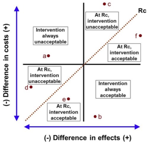
In this diagram, the dotted diagonal line marked Rc represents the ceiling ratio. If an intervention lies above the line, it will not be acceptable on cost-effectiveness grounds. This is either because it is dominated by the alternative, whatever
the ceiling ratio is, as in point A, or its ICER does not satisfy the actual ceiling ratio, as in points B and C. It should be noted that in the south-west quadrant, this means that the ICER is below the ceiling ratio, as in point B, while in the
north-east quadrant it is above, as in point C. Below the line it will be acceptable. This is either because it dominates the alternative, as in point D, or its ICER satisfies the ceiling ratio, as in points E and F. In this case, the ICER is above
the ceiling ratio in the south-west quadrant, as in point E, or below it in the north-east quadrant, as in point F.

Cost-effectiveness acceptability is also important because it is one way in which uncertainty in economic appraisal is dealt with – see section 5.6.1.

5.3.5 Cost-utility analysis (CUA)

Cost-utility analysis (CUA) is a term often used in the UK and elsewhere, though rarely in the United States, to refer to a special form of CEA in which health benefits are measured in terms of Quality-Adjusted-Life-Years (QALYs). QALYs are a
composite measure of gains in life expectancy and health-related quality of life that is discussed in more detail in section 5.5.1. The distinctive outcome of a CUA is the calculation for each an alternative of an ICER in terms of the extra cost per
QALY gained (CQG).

The rationale for CUA is more complex than that of CEA more generally. QALYs in themselves are regarded by many as a better outcome indicator than the ‘natural units’ of CEA when appraising therapeutic alternatives for the same condition. This
is beacuse they deal with efficiency in the production of health itself rather than simply of health care. But CUA offers something that CEA more generally cannot, which is the possibility of comparing across treatments for different conditions. In
principle, it is possible to compare treatments for, say, cancer with, say, physiotherapy to determine which is the most efficient at producing health gain in the form of QALYs. Of course, this is controversial. For a CEA restricted to different
treatments for a particular condition, it can be assumed that the patients receiving the treatments are the same people, but this will not be true of comparisons across conditions.

The ability that CUA has, in principle, to compare across all health interventions produces an even more contentious implication, which is that it can be used to allocate health care resources between them. The implication is that it can therefore
be used to determine health care priorities. That would overcome the principal problem that CEA has compared with CBA, because it would indicate whether or not the health care benefits from a particular type of health care should be realised, rather
than simply which is the best way of achieving those benefits. Some people therefore regard CUA as a limited form of CBA rather than a special form of CEA. Viewed in this way, CUA is better than CBA, because it avoids having to measure benefits in
terms of money.

To explain this further, recall that a decision rule for CEA is that the ICER of the best alternative is compared to a ceiling ratio. In the case of CUA the ICER is the CQG, so the ceiling ratio is the amount that we think it is reasonable to pay
to gain a QALY. This is sometimes referred to as a CQG threshold, because it is the dividing line between health care that is regarded as cost-effective and that which is not. The National Institute of Health and Clinical Excellence (NICE) has
a threshold, though it is not entirely clear what the size of that threshold is (Devlin and Parkin, 2004). The threshold could be regarded as deriving from the limited budget that the NHS has, which determines what can be afforded. This is known as
the shadow price of a QALY. Alternatively, it could be set according to what the population is willing to pay for health gain. This is known as the social value of a QALY. But either way, if this is known, it can in principle be used as
a means of converting costs to QALYs or vice versa. This puts costs and benefits into the same units, enabling the calculation of net benefits in the same way as for CBA.

Net benefits can either be calculated in terms of money or of QALYs. Suppose that an intervention has incremental costs of £30,000 and incremental benefits of 2 QALYs. The ceiling ratio can be regarded as the price that it is acceptable to pay
for a QALY, and therefore represents the money value of a QALY. Suppose that the ceiling ratio is £20,000 per QALY gained. If we decide to analyse cost-effectiveness in monetary terms, we first multiply the QALY gain by the ceiling ratio to give the
money value of the QALY gain, in this case 2x£20,000=£40,000. The net cost is then subtracted from this to give a net monetary benefit of £40,000-£30,000 = £10,000. Alternatively, we could convert the costs to their QALY gain equivalent
by dividing the ceiling ratio by them. This would give a net cost equivalent of £30,000/£20,000 = 1.5 QALYs, and an overall net health benefit of 2-1.5 = 0.5 QALYs. Because these are positive – and they must always have the same sign –
the intervention is deemed cost-effective.

Of course, this is exactly the same result as if we had calculated the ICER to be £30,000/2 = £15,000 and observed that it is below the ceiling ratio of £20,000. However, this net-benefit approach does have an advantage if we do not know the
ceiling ratio, since we can calculate net benefits for any value of the ceiling ratio, as illustrated in the following diagrams:

Net monetary benefit curve

Net health benefit curve

Like cost-effectiveness acceptability, this net benefit approach is also important because it is another way in which uncertainty in economic appraisal is dealt with – see section 5.6.1.

5.4 The measurement of costs

The theory of cost-benefit analysis suggests that

• all costs should be measured, whatever they are and whoever incurs them;
• costs should reflect opportunity costs; and
• marginal costs should be measured.

In practice, these theoretical principles are hard, if not impossible, to adhere to, but they still provide a guide as to what are the best sources of cost if there are alternatives and to the reliability of the numbers actually used.

The principle of looking at all costs is preserved in good practice in health economic appraisal by examining costs according to who bears them, in three categories: the health service, patients and their families, and the rest of society. The
principle that opportunity costs should be looked at is preserved in good practice by the separation of costing into use of resources and attaching a value to those resources to calculate costs; this is also good practice for ensuring that research
is generalisable. So, as suggested in section 5.2, the process of costing involves three steps:

1. Identifying and describing resource use changes.
2. Quantifying them in physical units.
3. Valuing them.

In general, there are two types of costing: – macro or ‘top-down’ costing and micro or ‘bottom-up’ costing. These are distinguished by the level of disaggregation at which individual resources are measured and valued. In
its pure form, macro costing starts with the total costs incurred by, for example, a hospital and calculates the costs of, for example a specialty, by allocating a proportion of the total costs to it using some indicator of the costliness of that
specialty compared with others. For example, if a specialty had 20% of the hospital’s cases, 20% of the costs would be allocated to it. At the extreme, micro-costing would examine every item of service and every consumable used by every patient.
Each item of service would be costed by examining all of the time spent on it by every member of staff as well as the time spent using every piece of equipment. In practice, these extremes are not found. Moreover, it is common for mixed methods to be
used for different elements of cost.

An important consideration is timing, as costs are incurred at a particular time and not all costs are incurred at the same time. There are two important elements to this. First, if costs occur in different years, then they should be adjusted for
any inflation or deflation that has occurred. This is to make the figures comparable over different years and to ensure that it is the value of resources that is considered, which may be unaffected by the rate of inflation. The best practice is to
select one year’s unit costs and apply them to different years’ resource use. But that is rarely possible for many items of cost, so the procedure is to deflate yearly costs by a cost index. This also means that if there are any cost projections,
these should not take account of projected inflation.

Secondly, although inflation-adjusting means that each year’s costs are measured in the same units of value for each year, this does not mean that every year’s costs are of the same value when viewed from a particular year. In particular,
people in general prefer to postpone costs if they can, and therefore a cost now has a higher weight than exactly the same money cost incurred in the future. Looked at another way, costs in the future have a lower value now. This is dealt with by discounting,
which is a time weight applied to costs, which diminishes the further in the future the cost is. In practice, what is done is to apply a discount rate, which can be viewed as the inverse of an interest rate. Applying an interest rate to an
investment means that the value grows over time even if it is fixed. Applying a discount rate means that the value falls over time. In an economic evaluation, if costs are summed over time, then discounting all future costs back to the present gives
a present value.

The issue of timing may be very important in health care, because of the long-lasting effects of many interventions. In particular, prevention incurs costs now, and even if it reduces costs in the future by a greater amount, there may not be a net
cost saving if the future costs are discounted. Even if there is a net cost savings, it will have a lower value than if discounting was not used. In the extreme, measures to deal with maternal nutrition to reduce illness in the later adult life of
their babies, as suggested by the Barker hypothesis (Barker, 1992), might see cost reductions so many years in the future that discounting would reduce them to a negligible value.

There is some dispute about exactly what the discount rate to be used should be, and how it should be obtained. There are two competing theories to guide this. One is the ‘social opportunity cost’ approach, which assumes that public and
private investments compete for resources, so the public sector should use market rates of borrowing. The other is the ‘social rate of time preference’, which measures what people are willing to receive in compensation for delaying consumption
from one year to the next. In practice, the discount rate in the UK is set by the Treasury in the Green Book referred to in section 5.3.2.

5.5 The measurement of benefits

Measurement of benefits in terms of ‘natural units’ in a CEA does not require any special economic analysis, and the measurement of diverse benefits within a CCA is too diverse to be dealt with here. This section therefore concentrates on the
measurement of health gain for use in a CUA, and the measurement of monetary gain for use in a CBA.

However, a technique that has recently been introduced which does not fit neatly into these two categories is conjoint analysis, which is becoming increasingly important. In this, respondents are offered a choice between different health
interventions, which are described according to ‘attributes’ that may include health outcomes and price. The choices made reveal the relative values of different attributes. This might be used to attribute a value to different health
interventions or to different health states or to calculate values in terms of money.

5.5.1 Measures of benefit in terms of health gain

There are many different ways in which health and improvements in health can be measured. Different concepts and measurement techniques are appropriate for different uses. The approaches that are adopted for use in economic appraisal are largely
determined by the requirements that their use for appraisal purposes dictates.

First, appraisal is attempting to obtain an unambiguous measure of benefit. This implies that the measure of health should be a single number representing all relevant aspects. Secondly, because appraisal looks at the use of scarce resources that
could be devoted to all sorts of health care, the measure of health should be capable of comparing those different uses of resources This implies that a ‘generic’ measure of health should be used. Thirdly, appraisal compares costs, which
represent the value of resources used with benefits. This implies that the measure of health should also be capable of being interpreted as a value.

One measure that meets these requirements is the Quality Adjusted Life Year (QALY). This combines length of life and quality of life into a single indicator. Depending on the type of health gain, QALYs can be thought of as a
quality adjustment to years of life gained or the length of time for which quality of life is improved or both. It is important to remember that the benefit of a health intervention is the gain in QALYs that it produces.

For example, suppose that with a particular disease, the prognosis is that a person will live for a further ten years; the first two of those will have a quality of life valued at 60% of full health and the last eight will have a quality of life
valued at 40%. With treatment, life expectancy will rise to 12 years, in each of which the patient will enjoy full health. The number of QALYs that the patient will have without treatment is (2x0.6) + (8x0.4) = 4.4. The number of QALYs that the
patient will have with treatment is (1x12) = 12. So, the benefit of the treatment is (12 – 4.4) = 7.6 QALYs gained.

One of the big advantages of the QALY is that it can, in principle, be applied to any kind of intervention, whether it raises life expectancy without improving quality of life, improves quality of life without affecting longevity, improves both or
improves one at the expense of lowering the other. However, to some people this is a weakness of QALYs, as they think that length and quality of life cannot or should not be compared in the same metric.

Before looking at how QALYs are calculated, it should be noted that if QALYs are gained, or indeed lost, at different times, then in principle they should be discounted if they are to be added together, in exactly the same way as costs, if they
are to be used in an economic evaluation. There has been a considerable debate about this and there are arguments in favour of discounting both costs and QALYs at the same rate, discounting costs but not QALYs, and discounting them both, but at
different rates. Current guidelines in the UK, for example from NICE, are to discount both at the same rate, that set by the Treasury.

In what follows, the concern is only with the quality of life element of the QALY, since the measurement of life expectancy has no special economic aspects attached to it.

In carrying out an appraisal, QALYs can be calculated in a number of different ways. One is to measure the value that patients attach to their quality of life directly. Another is to apply a conversion factor to other indicators of health that
will estimate from the indicator a quality of life value. However, an approach which has become most popular, and indeed is recommended by NICE, is to obtain from patients a measure of their health state using a generic health status measure, such as
the EQ-5D (Brooks, 1996), and to apply to the resulting health profile data a value for each state that has been measured for a different population. The intention is that those values should represent the values of society as a whole.

These sets of values are derived from population surveys. There are different techniques that are used to obtain values, of which the main three are Rating or Visual Analogue Scales, Time Trade-off and Standard Gamble.

A Visual Analogue Scale usually consists of a single line drawn with verbal and numerical descriptors at each end, describing the meaning of the two ends, such as ‘Best possible health’ and ‘Worst possible health’. Scale markers are
often added to the line to denote distance along the line, and these are sometimes also numbered. Respondents are presented with a set of health states and are asked to rate the desirability of each by placing it at some point on the line on or
between the two endpoints.

In the time trade-off method, respondents are offered a choice between a number of years in full health and a number of years in a particular health state and asked to choose between them. Slightly different versions of this are used
depending on whether the states are chronic or acute state and whether the respondent believes them to be better or worse than being dead. For a chronic health state preferred to death, different numbers of years in full health are offered for a
fixed number of years in a health state, until the respondent cannot choose between the alternatives. The value for the health state is then determined by the ratio of the number of years in full health to the number of years in the health state.
This calculation is based on the assumed equivalence of the number of QALYs generated by the two alternatives.

In the standard gamble method, respondents are offered a choice between the certainty of being in a particular health state and a gamble whose outcomes are full health with a certain probability and death, and asked to choose between them. Again,
slightly different versions of this are used depending on whether the states are chronic or acute and whether the respondent believes them to be better or worse than being dead. For a chronic health state preferred to death, different probabilities
of being in full health are offered, until the respondent cannot choose between the alternatives. The value for the health state is equal to the probability at that point of indifference. This calculation is based on the expected values of the
two alternatives, which is discussed in section 7.

Generic health state measures are usually accompanied by sets of values for the each health state that they define. Because they have so many health states, the values are usually generated by a model, which may be called a multi-attribute
utility model, though that label is not explicitly used in some cases and its use in some cases may be disputed. Essentially, health states are decomposed into ‘attributes’. Generic health measures usually describe health states using
different ‘dimensions’, in which people can be at different ‘levels’, which form the attributes. For example, the EQ-5D has the following dimensions and levels:

Mobility

1. No problems in walking about.
2. Some problems in walking about.
3. Confined to bed.

Self-care:

1. No problems with self-care.
2. Some problems washing or dressing self.
3. Unable to wash or dress self.

Usual activities

1. No problems with performing usual activities (e.g. work, study, housework).
2. Some problems with performing usual activities.
3. Unable to perform usual activities.

Pain and discomfort

1. No pain or discomfort.
2. Moderate pain or discomfort.
3. Extreme pain or discomfort.

Anxiety and depression

1. Not anxious or depressed.
2. Moderately anxious or depressed.
3. Extremely anxious or depressed.

The attributes, which in this case are levels within a particular dimension and interactions between the dimensions, are combined using a mathematical function. In the case of the EQ-5D, there are a number of value sets that have been calculated
and published, of which the most widely-known and used is taken from the UK Measuring and Valuing Health project undertaken at the University of York, based on the time trade-off method (Szende, Oppe and Devlin, 2007). The mathematical form used by
this is additive, which means that the attributes are weighted and added together.

5.5.2 Monetary measures of health benefits

Monetary measures of health benefits can be based on revealed preference or stated preference. Revealed preference techniques use observations from people’s behaviour to infer monetary values. As an example, it is possible to
examine the value that people place on the avoidance of death or injury by looking at the wages that are paid to people to undertake jobs that differ in the risk of these occurring but are otherwise identical. Revealed preference techniques, which
are increasingly used, rely on surveys and experiments in which people are essentially asked what monetary value is that they place on health states or on other aspects of health benefits. They are not asked that question directly, but are usually
given choices between different alternatives, whose descriptions include money values, from which money values are inferred.

Such revealed preference studies are sometimes called willingness-to-pay studies, although that description is not entirely accurate for all of them. The economic theory underlying these kinds of studies is the measurement of what are
called compensating variation and equivalent variation, which in this context means respectively monetary compensation made to a person for a change in health and monetary compensation to a person for not having a change in health. Willingness
to pay refers to compensation paid by the respondent, either for obtaining an improvement in their health or not having their health deteriorate. Willingness to accept refers to compensation paid to the respondent, either for
having their health deteriorate or not obtaining an improvement in their health.

Although methods used vary, best practice in economics more generally is to use the contingent valuation method. Contingent valuation requires the survey or experiment to describe a plausible market in which the choices made by respondents
about goods reveal the values that are required. The values are said to be contingent on that description.

5.6 Economic appraisal models and uncertainty

In theory, it is possible that an economic appraisal could be carried out using one source of data, for example a clinical trial in which resource use, costs and quality of life are all measured for individual patients. This would have all of the
advantages of a clinical trial in terms of the replicability of results. In practice, economic appraisals are usually based on different sources of data, which have to be linked together. There are many calculations behind the estimates of costs and
benefits, which are embodied in what is called an economic evaluation model, and in practice all health care appraisals involve some modelling. In fact, economic modelling is regarded by many as superior to a trial-based economic appraisal –
although models may use data from trials – as it may overcome the problems that trials have in terms of generalisability and slowness in producing usable results (Buxton et al, 1997; Halpern et al, 1998).

A simple model might be regarded simply as a balance sheet in which the data used to calculate costs and benefits are combined to give figures for total costs and total benefits. However, many economic appraisals cannot use such simple models, and
these are no longer regarded as acceptable in the context of technology appraisals examined by bodies such as NICE. The reasons are, first, that treatment options are not always straightforward and clinical decision making may involve strategies for
management, rather than a simple choice between using and not using a single therapy; and secondly, that there is usually some uncertainty about both the model and the data.

As a result, modelling usually uses decision analysis, which is described in section 7. This deals both with the complexity issue, by imposing a structure on the implied clinical decision making, and some aspects of uncertainty. However, there is
one aspect of uncertainty that is not dealt with directly by decision analysis, which is uncertainty about the values that data take. A number of techniques have been developed in recent years to deal with this, which are briefly described.

The problem that is dealt with can be encapsulated by the observation that summaries of effectiveness data, such as changes in blood pressure resulting from some intervention, are usually presented as both a point estimate and an interval
estimate, or confidence interval, reflecting variability in the data; we should have a similar summary for cost-effectiveness data. When this is done as part of a trial-based analysis it is called stochastic cost-effectiveness analysis.
Unfortunately, there are two problems with this. First, many of the data used in an appraisal model are not based on sampling, and therefore do not have a variance that can be used to create an interval estimate. Secondly, the summary index of
cost-effectiveness is the ICER, which as a ratio has special problems, such that in general it is not possible to estimate a confidence interval even if all of the data that are used to calculate it do have variability. This second problem applies
equally to trial-based and model based analyses.

5.6.1 Sensitivity analysis

The usual way in which uncertainty is dealt with when using a model is sensitivity analysis, which is a set of techniques that analyse how sensitive the results are to changes in the model, for example in the data that are contained within
it or the way that the data are combined. Some sensitivity analysis techniques are described below. In these, the model that has the best assumed structure and data is called the base case, and the assumptions and data that we wish to test are
referred to as the parameters of the model.

One-way sensitivity analysis means looking at how sensitive results are to changes in one parameter. If, for example, a new drug therapy is appraised using a model, one of the parameters of the model may be the unit cost of the drug. The
base case will use the best estimate that the analyst has of the unit cost as an input to the calculated ICER. One-way sensitivity analysis will calculate the ICER for different values of the unit costs, showing whether the cost makes a lot or a
little difference to the result.

Of course, what is meant by ‘a lot’ or ‘a little’ should really be defined. One way to do this is to use the ceiling ratio. If at every possible value of the parameter the ICER remains above or alternatively remains below the ceiling
ratio, then the result remains the same, and the decision is not sensitive to the value of the uncertain parameter. In other cases, it may be that at some levels of the parameter – for example when the unit cost is low - the ICER will be below the
ceiling ratio, but at others - for example when the unit cost is high – the ICER will be above. At some point the CER will be equal to the ceiling ratio, and at that point –called a threshold - a change in the preferred option occurs. This is
known as threshold analysis. If the base case and the threshold are very different, then the results are not sensitive to the values of the parameter.

But again, what does ‘very different’ mean? One way to deal with this is to define upper and lower plausible values for the parameter – for example with a base case cost of £100 per unit, it may be thought unlikely that the cost could be as
high as £200 or as low as £10. This will give a plausible range to the calculated ICER, and if the threshold is within that range, then the results are sensitive to the assumption made.

This can be extended to vary more than one parameter at the same time and to observe the combined impact on the ICER. The ceiling ratio can again be used to define a threshold, and plausible ranges for the ICER can be calculated from the plausible
values of the variables, taken in combination. Such multi-way analysis is essential, because it is possible that separate one way analyses of the parameters might suggest that the results are not sensitive to their value, but in combination they
might be.

5.6.2 Statistical sensitivity analysis

Plausible range methods are not very satisfactory because their basis is often unclear and not testable. Using statistical methods are better because, as suggested, the base case cost-effectiveness results can be seen as a point estimate and
sensitivity analysis as an interval estimate. When this is done as part of a decision analysis model, it is called probabilistic sensitivity analysis.

In this, Monte Carlo simulations are used to generate an ICER distribution. A distribution for each of the model’s parameters is assumed, if it is not known. Samples are taken from each distribution, and the ICER is calculated from those
simulated data using the model. This is repeated many times to generate an ICER distribution, from which, in principle, a variance might be calculated, and therefore a confidence interval.

Unfortunately, in practice that might still not be possible, because of another problem with ICERs. It is quite possible that their distribution might spread over more than one quadrant of the CE plane. Values for the ICERs generated by simulation
may include both positive and negative values. These mean such different things that a confidence interval calculated from them is meaningless.

There are two possible solutions to this. One is essentially to get rid of the ICER by using the net benefit approach described earlier. Because net benefit is a single number, not a ratio, there is no problem with using simulation to generate a
distribution of it and to calculate a variance and therefore an interval estimate.

Another solution is to generate a cost-effectiveness acceptability curve (CEAC), which retains the CER, but gets rid of the need to have a confidence interval to describe uncertainty. The simulated ICER values are each compared with a
ceiling ratio, and a count is obtained of the proportion of simulated values that are acceptable at that ratio. This is repeated for each possible value of the ceiling ratio, and the proportion that is acceptable will be different for each of those
values. A CEAC plots these together, as in this diagram:

In this diagram, the proportion that is cost-effective is labelled the probability that the intervention is cost-effective. However, that interpretation is only true under certain circumstances, essentially a Bayesian interpretation that is beyond
the scope of this document.

© David Parkin 2009