
Sampling Distributions
Statistics: Significance testing, Type I and Type II errors
This section covers:
- Significance Testing
- P-values
- Type I Errors
- Type II errors
- Power
- Sample size estimation
- Problems of multiple testing
- Bonferroni correction
Consider the data below in Table 1, given in Campbell and Swinscow (2009).
A general practitioner wants to compare the mean of the printers' blood pressures with the mean of the farmers' blood pressures.
Table 1 Mean diastolic blood pressures of printers and farmers

Null hypothesis and type I error
In comparing the mean blood pressures of the printers and the farmers we are testing the hypothesis that the two samples came from the same population of blood pressures. The hypothesis that there is no difference between the population from which the printers' blood pressures were drawn and the population from which the farmers' blood pressures were drawn is called the null hypothesis.
But what do we mean by "no difference"? Chance alone will almost certainly ensure that there is some difference between the sample means, for they are most unlikely to be identical. Consequently, we set limits within which we shall regard the samples as not having any significant difference. If we set the limits at twice the standard error of the difference, and regard a mean outside this range as coming from another population, we shall on average be wrong about one time in 20 if the null hypothesis is in fact true. If we do obtain a mean difference bigger than two standard errors we are faced with two choices: either an unusual event has happened, or the null hypothesis is incorrect. Imagine tossing a coin five times and getting the same face each time. This has nearly the same probability (6.3%) as obtaining a mean difference bigger than two standard errors when the null hypothesis is true. Do we regard it as a lucky event or suspect a biased coin? If we are unwilling to believe in unlucky events, we reject the null hypothesis, in this case that the coin is a fair one.
To reject the null hypothesis when it is true is to make what is known as a type I error. The level at which a result is declared significant is known as the type I error rate, often denoted by α. We try to show that a null hypothesis is unlikely, not its converse (that it is likely), so a difference which is greater than the limits we have set, and which we therefore regard as "significant", makes the null hypothesis unlikely. However, a difference within the limits we have set, and which we therefore regard as "non-significant", does not make the hypothesis likely. To repeat an old adage, 'absence of evidence is not evidence of absence'.
A range of not more than two standard errors is often taken as implying "no difference" but there is nothing to stop investigators choosing a range of three standard errors (or more) if they want to reduce the chances of a type I error.
Testing for differences of two means
In testing whether the difference in blood pressure of printers and farmers could have arisen by chance, the general practitioner seeks to reject the null hypothesis that there is no significant difference between them. The question is, how many multiples of its standard error does the difference in means represent? Since the difference in means is 9 mmHg and its standard error is 0.81 mmHg, the answer is: 9/0.805=11.2. We usually denote the ratio of an estimate to its standard error by "z", that is, z = 11.2. Reference to Normal Tables shows that z is far beyond the figure of 3.291 standard deviations, representing a probability of 0.001 (or 1 in 1000). The probability of a difference of 11.2 standard errors or more occurring by chance is therefore exceedingly low, and correspondingly the null hypothesis that these two samples came from the same population of observations is exceedingly unlikely. This probability is known as the P value and may be written P.
It is worth recapping this procedure, which is at the heart of statistical inference. Suppose that we have samples from two groups of subjects, and we wish to see if they could plausibly come from the same population. The first approach would be to calculate the difference between two statistics (such as the means of the two groups) and calculate the 95% confidence interval. If the two samples were from the same population we would expect the confidence interval to include zero 95% of the time, and so if the confidence interval excludes zero we suspect that they are from a different population. The other approach is to compute the probability of getting the observed value, or one that is more extreme, if the null hypothesis were correct. This is the P value. If this is less than a specified level (usually 5%) then the result is declared significant and the null hypothesis is rejected. These two approaches, the estimation and hypothesis testing approach, are complementary. Imagine if the 95% confidence interval just captured the value zero, what would be the P value? A moment's thought should convince one that it is 2.5%. This is known as a one-sided P value, because it is the probability of getting the observed result or one bigger than it. However, the 95% confidence interval is two sided, because it excludes not only the 2.5% above the upper limit but also the 2.5% below the lower limit. To support the complementarity of the confidence interval approach and the null hypothesis testing approach, most authorities double the one sided P value to obtain a two sided P value.
Alternative hypothesis and type II error
It is important to realise that when we are comparing two groups a non-significant result does not mean that we have proved the two samples come from the same population - it simply means that we have failed to prove that they do not come from the population. When planning studies it is useful to think of what differences are likely to arise between the two groups, or what would be clinically worthwhile; for example, what do we expect to be the improved benefit from a new treatment in a clinical trial? This leads to a study hypothesis, which is a difference we would like to demonstrate. To contrast the study hypothesis with the null hypothesis, it is often called the alternative hypothesis. If we do not reject the null hypothesis when in fact there is a difference between the groups we make what is known as a type II error. The type II error rate is often denoted as β. The power of a study is defined as 1-β and is the probability of rejecting the null hypothesis when it is false. The most common reason for type II errors is that the study is too small.
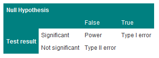
The relationship between Type I and Type II errors is shown in Table 2. One has to imagine a series of cases, in some of which the null hypothesis is true and in some of which it is false. In either situation we carry out a significance test, which sometimes is significant and sometimes not.
The concept of power is only relevant when a study is being planned. After a study has been completed, we wish to make statements not about hypothetical alternative hypotheses but about the data, and the way to do this is with estimates and confidence intervals.
Table 2 Relationship between Type I and Type II errors
Steps to calculating sample size
Usually the significance level is predefined (5% or 1%).
Select the power you want the study to have, usually 80% or 90% (i.e. type II error of 10-20%)
For continuous data, obtain the standard deviation of the outcome measure.
For binary data, obtain the incidence of the outcome in the control group (for a trial) or in the non-exposed group (for a case-control study or cohort study).
Choose an effect size. This is the size of the effect that would be 'clinically' meaningful.
For example, in a clinical trial, the sort of effect that would make it worthwhile changing treatments. In a cohort study, the size of risk that implies a public hazard.
Use sample size tables or a computer program to deduce the required sample size.
Often some negotiation is required to balance the power, effect size and an achievable sample size.
One should always adjust the required sample size upwards to allow for dropouts.
Problems of multiple testing
Imagine carrying out 20 trials of an inert drug against placebo. There is a high chance that at least one will be statistically significant. It is highly likely that this is the one which will be published and the others will languish unreported. This is one aspect of publication bias. The problem of multiple testing happens when:
1. Many outcomes are tested for significance
2. In a trial, one outcome is tested a number of times during the follow up
3. Many similar studies are being carried out at the same time.
The ways to combat this are:
1. To specify clearly in the protocol which are the primary outcomes (few in number) and which are the secondary outcomes.
2. To specify at which time interim analyses are being carried out, and to allow for multiple testing.
3. To do a careful review of all published and also unpublished studies. Of course, the latter, by definition, are harder to find.
A useful technique is the Bonferroni correction. This states that if one is doing n independent tests one should specify the type I error rate as α/n rather than α. Thus, if one has 10 independent outcomes, one should declare a significant result only if the p-value attached to one of them is less than 5%/10, or 0.5%. This test is conservative, i.e. less likely to give a significant result because tests are rarely independent. It is usually used informally, as a rule of thumb, to help decide if something which appears unusual is in fact quite likely to have happened by chance.
Reference
- Campbell MJ and Swinscow TDV. Statistics at Square One 11th ed. Wiley-Blackwell: BMJ Books 2009. Chapter 6.
© MJ Campbell 2016, S Shantikumar 2016