
Statistics: Reference ranges, standard errors and confidence intervals
Standard error of the mean
A series of samples drawn from one population will not be identical. They will show chance variations from one to another, and the variation may be slight or considerable. For example, a series of samples of the body temperature of healthy people would show very little variation from one to another, but the variation between samples of the systolic blood pressure would be considerable. Thus, the variation between samples depends partly on the amount of variation in the population from which they are drawn.
Furthermore, it is a matter of common observation that a small sample is a much less certain guide to the population from which it was drawn than a large sample. In other words, the more members of a population that are included in a sample the more chance that sample will have of accurately representing the population, provided a random process is used to construct the sample. A consequence of this is that, if two or more samples are drawn from a population, the larger they are the more likely they are to resemble each other - again provided that the random technique is followed. Thus, the variation between samples depends partly also on the size of the sample.
If we draw a series of samples and calculate the mean of the observations in each, we have a series of means. These means generally conform to a Normal distribution, and they often do so even if the observations from which they were obtained do not. This can be proven mathematically and is known as the "Central Limit Theorem". The series of means, like the series of observations in each sample, has a standard deviation. The standard error of the mean of one sample is an estimate of the standard deviation that would be obtained from the means of a large number of samples drawn from that population.
As noted above, if random samples are drawn from a population their means will vary from one to another. The variation depends on the variation of the population and the size of the sample. We do not know the variation in the population so we use the variation in the sample as an estimate of it. This is expressed in the standard deviation.
To derive an estimate of the standard error of the mean (SEM), we divide the standard deviation (SD) by the square root of the number of observations, as follows
\({\rm{SEM}} = \frac{{{\rm{SD}}}}{{\sqrt n }}\)
It is important to realise that we do not have to take repeated samples in order to estimate the standard error; there is sufficient information within a single sample. However, the conception is that if we were to take repeated random samples from the population, this is how we would expect the mean to vary, purely by chance.
Example
A general practitioner has been investigating whether the diastolic blood pressure of men aged 20-44 differs between the printers and the farm workers. For this purpose she has obtained a random sample of 72 printers and 48 farm workers and calculated the mean and standard deviations, as shown in Table 1.
Table 1 Mean diastolic blood pressures of printers and farmers
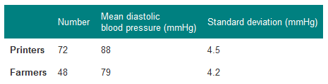
To calculate the standard errors of the two mean blood pressures the standard deviation of each sample is divided by the square root of the number of the observations in the sample.
Printers: SEM=4.5/√72=0.53 mmHg
Farmers: SEM=4.2/√48=0.61 mmHg
These standard errors may be used to study the significance of the difference between the two means.
Standard error of a proportion or a percentage
Just as we can calculate a standard error associated with a mean so we can also calculate a standard error associated with a percentage or a proportion. Here the size of the sample will affect the size of the standard error but the amount of variation is determined by the value of the percentage or proportion in the population itself, and so we do not need an estimate of the standard deviation. For example, a senior surgical registrar in a large hospital is investigating acute appendicitis in people aged 65 and over. As a preliminary study he examines the hospital case notes over the previous 10 years and finds that of 120 patients in this age group with a diagnosis confirmed at operation 73 (60.8%) were women and 47(39.2%) were men.
If p represents one percentage, 100-p represents the other. Then the standard error (SE) of each of these percentages is obtained by (1) multiplying them together, (2) dividing the product by the number in the sample, and (3) taking the square root:
\({\rm{SE\;percentage}} = {\rm{\;}}\sqrt {\frac{{p\;\left( {100 - p} \right)}}{n}}\)
which for the appendicitis data given above is as follows:
\({\rm{SE\;percentage}} = {\rm{\;}}\sqrt {\frac{{60.8 \times 39.2}}{{120}}}\)
Note that the above formula uses percentages. If you are given proportions, you can either convert these to percentages (multiply by 100), or use the modified formula below:
\({\rm{SE\;proportion}} = {\rm{\;}}\sqrt {\frac{{p\;\left( {1 - p} \right)}}{n}}\)
Standard error of count data
Standard errors can also be calculated for count data, where you are given a number of events over set period of time. Examples include the number of cardiac arrests in an A&E department every year, or the number referral rate from primary care to a specialist service per 1,000 patients per year. The standard error of a count (often denoted λ) is given by:
\({\rm{SE\;count}} = {\rm{\;}}\sqrt \lambda\)
For example, a GP in a busy practice sees 36 patients in a given day. The standard error is therefore √36 = 6.
Pooling standard errors of two groups
In the previous three sections, we calculated the standard error of a single group. In practice, we often want to compare two groups, commonly to determine whether or not they are different. One way of comparing two groups is to look at the difference (in means, proportions or counts) and constructing a 95% confidence interval for the difference (see below). As part of this process, we are required to calculate a pooled standard error of the two groups. The formulae required are similar to those given above, only this time each calculation within the square root is done twice, once for each group, before the square root is applied. This can be seen by comparing the formulae below:
One group Difference betweentwo groups
SE mean \(\frac{{SD}}{{\sqrt n }}\;\;or\;\sqrt {\frac{{SD_\;^2}}{{{n_\;}}}}\) \(\sqrt {\frac{{SD_1^2}}{{{n_1}}} + \frac{{SD_2^2}}{{{n_2}}}}\)
SE proportion \({\rm{\;}}\sqrt {\frac{{p{\rm{\;}}\left( {1 - p} \right)}}{n}}\) \({\rm{\;}}\sqrt {\frac{{{p_1}{\rm{\;}}\left( {1 - {p_1}} \right)}}{{{n_1}}} + \frac{{{p_2}{\rm{\;}}\left( {1 - {p_2}} \right)}}{{{n_2}}}}\)
SE count \(√ λ \) \({\rm{\;}}\sqrt {{\lambda _1} + \;{\lambda _2}\;}\)
The subscripts 1 and 2 relate to the estimates from groups 1 and 2. Note that, although these standard errors relate to the difference between two means/proportions/counts, the pooled standard errors are created by addition.
Reference ranges
Campbell and Swinscow (2009) describe 140 children who had a mean urinary lead concentration of 2.18 μmol/24h, with standard deviation 0.87. The points that include 95% of the observations are 2.18+/-(1.96x0.87), giving an interval of 0.48 to 3.89. One of the children had a urinary lead concentration of just over 4.0 μmol/24h. This observation is greater than 3.89 and so falls in the 5% beyond the 95% probability limits. We can say that the probability of each of such observations occurring is 5%. Another way of looking at this is to see that if one chose one child at random out of the 140, the chance that their urinary lead concentration exceeded 3.89, or was less than 0.48, is 5%. This probability is usually expressed as a fraction of 1 rather than of 100, and written P.
Standard deviations thus set limits about which probability statements can be made. Some of these are set out in Table 2.
Table 2 Probabilities of multiples of standard deviation for a Normal distribution
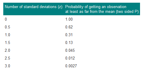
The probabilities set out in Table 2 can be used to estimate the probability of finding an observed value. For example, if we want to estimate the probability for finding a urinary lead concentration of 4.8 μmol/24h if sampling from the same population of observations as the 140 children provided, we proceed as follows. The distance of the new observation from the mean is 4.8-2.18=2.62. How many standard deviations does this represent? Dividing the difference by the standard deviation gives 2.62/0.87=3.01. Table 2 shows that the probability is very close to 0.0027. This probability is small, so the observation probably did not come from the same population as the 140 other children.
To take another example, the mean diastolic blood pressure of printers was found to be 88mmHg and the standard deviation 4.5 mmHg. One of the printers had a diastolic blood pressure of 100mmHg. The mean plus or minus 1.96 times its standard deviation gives the following two figures:
88 + (1.96 x 4.5) = 96.8 mmHg
88 - (1.96 x 4.5) = 79.2 mmHg.
We can say therefore that only 1 in 20 (or 5%) of printers in the population from which the sample is drawn would be expected to have a diastolic blood pressure below 79 or above about 97mmHg. These are the 95% limits. The 99.73% limits lie three standard deviations below and three above the mean. The blood pressure of 100mmHg noted in one printer thus lies beyond the 95% limit of 97 but within the 99.73% limit of 101.5 (=88+(3x4.5)).
The 95% limits are often referred to as a "reference range". For many biological variables, they define what is regarded as the normal (meaning standard or typical) range. Anything outside the range is regarded as abnormal. Given a sample of disease-free subjects, an alternative method of defining a normal range would be simply to define points that exclude 2.5% of subjects at the top end and 2.5% of subjects at the lower end. This would give an empirical normal range. Thus in the 140 children we might choose to exclude the three highest and three lowest values. However, it is much more efficient to use the mean +/-2SD, unless the data set is quite large (say >400).
Confidence intervals
The means and their standard errors can be treated in a similar fashion. If a series of samples are drawn and the mean of each calculated, 95% of the means would be expected to fall within the range of two standard errors above and two below the mean of these means. This common mean would be expected to lie very close to the mean of the population. So the standard error of a mean provides a statement of probability about the difference between the mean of the population and the mean of the sample.
In our sample of 72 printers, the standard error of the mean was 0.53 mmHg. The sample mean plus or minus 1.96 times its standard error gives the following two figures:
88 + (1.96 x 0.53) = 89.04 mmHg
88 - (1.96 x 0.53) = 86.96 mmHg.
This is called the 95% confidence interval (95% CI), and we can say that there is only a 5% chance that the range 86.96 to 89.04 mmHg excludes the mean of the population. If we take the mean plus or minus three times its standard error, the interval would be 86.41 to 89.59. This is the 99.73% confidence interval, and the chance of this interval excluding the population mean is 1 in 370 (i.e. 0.27%). Confidence intervals provide the key to a useful device for arguing from a sample back to the population from which it came. They are discussed further in Standard Statistical Distributions (e.g. Normal, Poisson, Binomial) and their uses
With small samples - say fewer than 30 observations - larger multiples of the standard error are needed to set confidence limits. This subject is discussed under the t distribution.
Confidence interval for a proportion
In a survey, of 120 people operated on for appendicitis, 47 were men.
The standard error for the proportion of male patients with appendicitis, is given by:
\({\rm{SE\;}}\left( p \right) = {\rm{\;}}\sqrt {\frac{{p\;\left( {1 - p} \right)}}{n}} = \;{\rm{\;}}\sqrt {\frac{{\frac{{47}}{{120}}\;\left( {1 - \frac{{47}}{{120}}} \right)}}{{120}}} = 0.0446\;\left( {or\;4.46\% } \right)\)
Note that this is also the standard error of the percentage of female patients with appendicitis, since the calculation remains the same if p is replaced by 1-p. Using this standard error we can get 95% confidence intervals on the two percentages:
95% CI for proportion of females 60.8 ± (1.96 x 4.46) = 52.1 and 69.5
95% CI for proportion of males 39.2 ± (1.96 x 4.46) = 30.5 and 47.9.
These confidence intervals exclude 50%, which would be the expected values if appendicitis was equally common in males and females in this population. We can conclude that females are more likely to get appendicitis than males. This formula is only approximate, and works best if n is large and p is between 0.1 and 0.9.
There is much confusion over the interpretation of the probability attached to confidence intervals. To understand it we have to resort to the concept of repeated sampling. Imagine taking repeated samples of the same size from the same population. For each sample calculate a 95% confidence interval. Since the samples are different, so are the confidence intervals. We know that 95% of these intervals will include the population parameter. However, without any additional information we cannot say which ones! Thus, with only one sample, and no other information about the population parameter, we can say there is a 95% chance of including the parameter in our interval. Note that this does not mean that we would expect with 95% probability that the mean from another sample is in this interval.
General formulae for confidence intervals
As demonstrated from the examples above, the same approach is used to construct confidence intervals. In general, a 95% confidence interval is calculated as follows:
95% CI = estimate ± (1.96 x SE)
…where the estimate could be mean, proportion or count, and where the standard error (SE) is calculated using the relevant formula. In the equation above, the numerical value 1.96 relates to the 95% confidence level. Other commonly used limits are the 90% and 99% confidence interval, in which case the 1.96 may be replaced by 1.65 (for 90%) or 2.58 (for 99%).
A similar general formula can be used to determine the confidence intervals for the difference between two estimates, as follows:
95% CI for a difference = (difference between two estimates) ± (1.96 x pooled SE)
…again, where the estimates may be means, proportions or counts, and where the pooled SE is calculated using the relevant formula.
Example
The prevalence of teenage pregnancies in a city was 49 per 1000 in 2005 and 25 per 1000 in 2015. To determine if this reduction is significant, we have two options. Either we can calculate the confidence intervals for each of the two prevalence rates separately and compare them, or we can calculate a confidence interval for the difference between the two estimates.
These are count data, and we will use the relevant standard error formula given above. Using the first option, we calculate 95% confidence intervals for the prevalence of teenage pregnancy in 2005 and 2015:
95% CI in 2005 = 49 ± (1.96 x √49) = (35.3, 62.7)
95% CI in 2015 = 25 ± (1.96 x √25) = (15.2, 34.8)
Because these two confidence intervals do not overlap, we can infer that there is a significant difference between the two prevalence rates. Specifically, there has been a significant reduction in the prevalence of teenage pregnancy between 2005 and 2015 (at the 95% level).
Now we will use the second approach – calculating the difference between the two prevalence rates. We first calculate the pooled standard error, followed by the 95% confidence interval, as follows:
\({\rm{Pooled\;SE}} = {\rm{\;\;}}\sqrt {{\lambda _1} + \;{\lambda _2}\;} = \;\sqrt {49 + \;25\;} = 8.6\)
\(95{\rm{\% \;CI\;for\;difference}} = ({\lambda _1} - \;{\lambda _2})\)
= (49 – 25) ± (1.96 x 8.6) = (7.1, 40.9)
As this confidence interval does not include the value of no difference (i.e. zero), then we can conclude that there is a significant difference between the two prevalence rates (as was found using the previous method). We can see that using either of the above methods results in the same conclusion.
What is the difference between a reference range and a confidence interval?
There is precisely the same relationship between a reference range and a confidence interval as between the standard deviation and the standard error. The reference range refers to individuals and the confidence intervals to estimates. It is important to realise that samples are not unique. Different investigators taking samples from the same population will obtain different estimates of the population parameter, and have different 95% confidence intervals. However, we know that for 95 of every 100 investigators the confidence interval will include the population parameter (we just don't know which ones).
References
BMJ Statistics NoteStandard deviations and standard errors Altman DG Bland JM (2005)
http://bmj.bmjjournals.com/cgi/content/full/331/7521/903
- Campbell MJ and Swinscow TDV. Statistics at Square One 11th ed. Wiley-Blackwell: BMJ Books 2009. Chapter 5.
© MJ Campbell 2016, S Shantikumar 2016