
Statistics: Elementary Probability Theory
A probability gives the likelihood that a defined event will occur. It is quantified as a positive number between 0 (the event is impossible) and 1 (the event is certain). Thus, the higher the probability of a given event, the more likely it is to occur. If A is a defined event, then the probability of A occurring is expressed as P(A). Probability can be expressed in a number of ways. A frequentist approach is to observe a number of particular events out of a total number of events. Thus, we might say the probability of a boy is 0.52, because out of a large number of singleton births we observe 52% are boys. A model based approach is where a model, or mechanism determines the event; thus, the probability of a ‘1’ from an unbiased die is 1/6 since there are 6 possibilities, each equally likely and all adding to one. An opinion based approach is where we use our past experience to predict a future event, so we might give the probability of our favourite football team winning the next match, or whether it will rain tomorrow.
Given two events A and B, we often want to determine the probability of either event, or both events, occurring.
Addition Rule
The addition rule is used to determine the probability of at least one of two (or more) events occurring. In general, the probability of either event A or B is given by:
P(A or B) = P(A) + P(B) – P(A and B)
If A and B are mutually exclusive, this means they cannot occur together, i.e. P(A and B)=0. Therefore, for mutually exclusive events the probability of either A or B occurring is given by:
P(A or B) = P(A) + P(B)
Example: If event A is that a person is blood group O and event B is that they are blood group B, then these events are mutually exclusive since a person may only be either one or the other. Hence, the probability that a given person is either group O or B is P(A)+P(B).
Multiplication Rule
The multiplication rule gives the probability that two (or more) events happen together. In general, the probability of both events A and B occurring is given by:
P(A and B) = P(A) x P(B|A) = P(B) x P(A|B)
The notation P(B|A) is the probability that event B occurs given that event A has occurred where the symbol ‘|’ is read is ‘given’. This is an example of a conditional probability, the condition being that event A has happened. For example, the probability of drawing the ace of hearts from a well shuffled pack is 1/51. The probability of the ace of hearts given that the card is red is 1/26.
Example: If event A is a person getting neuropathy and event B that they are diabetic, then P(A|B) is the probability of getting neuropathy given that they are diabetic.
If A and B are independent events, then the probability of event B is unaffected by the probability of event A (and vice versa). In other words, P(B|A) = P(B). Therefore, for independent events, the probability of both events A and B occurring is given by:
P(A and B) = P(A) x P(B)
Example: If event A is that a person is blood group O and event B that they are diabetic, then the probability of someone having blood group O and being diabetic is P(A)xP(B), assuming that getting diabetes is unrelated to a person’s blood group.
Note that if A and B are mutually exclusive, then P(A|B)=0
Bayes’ Theorem
From the multiplication rule above, we see that:
P(A) x P(B|A) = P(B) x P(A|B)
This leads to what is known as Bayes' theorem:
\({\rm{P}}\left( {{\rm{B|A}}} \right) = {\rm{\;}}\frac{{{\rm{P}}\left( {{\rm{A|B}}} \right){\rm{P}}\left( {\rm{B}} \right)}}{{{\rm{P}}\left( {\rm{A}} \right)}}\)
Thus, the probability of B given A is the probability of A given B, times the probability of B divided by the probability of A.
This formula is not appropriate if P(A)=0, that is if A is an event which cannot happen.
An example of the use of Bayes’ theorem is given below.
Sensitivity and Specificity
Many diagnostic test results are given in the form of a continuous variable (that is one that can take any value within a given range), such as diastolic blood pressure or haemoglobin level. However, for ease of discussion we will first assume that these have been divided into positive or negative results. For example, a positive diagnostic result of 'hypertension' is a diastolic blood pressure greater than 90 mmHg; whereas for 'anaemia', a haemoglobin level less than 12 g/dl is required.
For every diagnostic procedure (which may involve a laboratory test of a sample taken) there is a set of fundamental questions that should be asked. Firstly, if the disease is present, what is the probability that the test result will be positive? This leads to the notion of the sensitivity of the test. Secondly, if the disease is absent, what is the probability that the test result will be negative? This question refers to the specificity of the test. These questions can be answered only if it is known what the 'true' diagnosis is. In the case of organic disease this can be determined by biopsy or, for example, an expensive and risky procedure such as angiography for heart disease. In other situations it may be by 'expert' opinion. Such tests provide the so-called 'gold standard'.
Example
Consider the results of an assay of N-terminal pro-brain natriuretic peptide (NT-proBNP) for the diagnosis of heart failure in a general population survey in those over 45 years of age, and in patients with an existing diagnosis of heart failure, obtained by Hobbs, Davis, Roalfe, et al (BMJ 2002) and summarised in table 1. Heart failure was identified when NT-proBNP > 36 pmol/l.
Table 1: Results of NT-proBNP assay in the general population over 45 and those with a previous diagnosis of heart failure (after Hobbs, David, Roalfe et al, BMJ 2002)
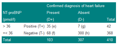
We denote a positive test result by T+, and a positive diagnosis of heart failure (the disease) by D+. The prevalence of heart failure in these subjects is 103/410=0.251, or approximately 25%. Thus, the probability of a subject chosen at random from the combined group having the disease is estimated to be 0.251. We can write this as P(D+)=0.251.
The sensitivity of a test is the proportion of those with the disease who also have a positive test result. Thus the sensitivity is given by e/(e+f)=35/103=0.340 or 34%. Now sensitivity is the probability of a positive test result (event T+) given that the disease is present (event D+) and can be written as P(T+|D+), where the '|' is read as 'given'.
The specificity of the test is the proportion of those without disease who give a negative test result. Thus the specificity is h/(g+h)=300/307=0.977 or 98%. Now specificity is the probability of a negative test result (event T-) given that the disease is absent (event D-) and can be written as P(T-|D-).
Since sensitivity is conditional on the disease being present, and specificity on the disease being absent, in theory, they are unaffected by disease prevalence. For example, if we doubled the number of subjects with true heart failure from 103 to 206 in Table 1, so that the prevalence was now 103/(410+103)=20%, then we could expect twice as many subjects to give a positive test result. Thus 2x35=70 would have a positive result. In this case the sensitivity would be 70/206=0.34, which is unchanged from the previous value. A similar result is obtained for specificity.
Sensitivity and specificity are useful statistics because they will yield consistent results for the diagnostic test in a variety of patient groups with different disease prevalences. This is an important point; sensitivity and specificity are characteristics of the test, not the population to which the test is applied. In practice, however, if the disease is very rare, the accuracy with which one can estimate the sensitivity may be limited. This is because the numbers of subjects with the disease may be small, and in this case the proportion correctly diagnosed will have considerable uncertainty attached to it.
Two other terms in common use are: the false negative rate (or probability of a false negative) which is given by f/(e+f)=1-sensitivity, and the false positive rate (or probability of a false positive) or g/(g+h)=1-specificity.
These concepts are summarised in Table 2.
Table 2: Summary of definitions of sensitivity and specificity
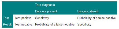
It is important for consistency always to put true diagnosis on the top, and test result down the side. Since sensitivity=1–P(false negative) and specificity=1–P(false positive), a possibly useful mnemonic to recall this is that 'sensitivity' and 'negative' have 'n's in them and 'specificity' and 'positive' have 'p's in them.
Predictive Value of a Test
Suppose a doctor is confronted by a patient with chest pain suggestive of angina, and that the results of the study described in Table 3 are available.
Table 3: Results of exercise tolerance test in patients with suspected coronary artery disease
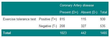
The prevalence of coronary artery disease in these patients is 1023/1465=0.70. The doctor therefore believes that the patient has coronary artery disease with probability 0.70. In terms of betting, one would be willing to lay odds of about 7:3 that the patient does have coronary artery disease. The patient now takes the exercise test and the result is positive. How does this modify the odds? It is first necessary to calculate the probability of the patient having the disease, given a positive test result. From Table 3, there are 930 men with a positive test, of whom 815 have coronary artery disease. Thus, the estimate of 0.70 for the patient is adjusted upwards to the probability of disease, with a positive test result, of 815/930=0.88.
This gives the predictive value of a positive test (positive predictive value):
P(D+|T+) = 0.88.
The predictive value of a negative test (negative predictive value) is:
P(D-|T-) = 327/535 = 0.61.
These values are affected by the prevalence of the disease. For example, if those with the disease doubled in Table 3, then the predictive value of a positive test would then become 1630/(1630+115)=0.93 and the predictive value of a negative test 327/(327+416)=0.44.
The Role of Bayes' Theorem
Suppose event A occurs when the exercise test is positive and event B occurs when angiography is positive. The probability of having both a positive exercise test and coronary artery disease is thus P(T+ and D+). From Table 3, the probability of picking out one man with both a positive exercise test and coronary heart disease from the group of 1465 men is 815/1465=0.56.
However, from the multiplication rule:
P(T+ and D+) = P(T+|D+)P(D+)
P(T+|D+)=0.80 is the sensitivity of the test and P(D+)=0.70 is the prevalence of coronary disease and so P(T+ and D+)=0.80x0.70=0.56, as before.
Bayes' theorem enables the predictive value of a positive test to be related to the sensitivity of the test, and the predictive value of a negative test to be related to the specificity of the test. Bayes' theorem enables prior assessments about the chances of a diagnosis to be combined with the eventual test results to obtain a so-called “posterior” assessment about the diagnosis. It reflects the procedure of making a clinical judgement.
In terms of Bayes' theorem, the diagnostic process is summarised by:
\({\rm{P}}\left( {{\rm{D}} + {\rm{|T}} + } \right) = {\rm{\;}}\frac{{{\rm{P}}({\rm{T}} + |{\rm{D}} + ){\rm{P}}\left( {{\rm{D}} + } \right)}}{{{\rm{P}}\left( {{\rm{T}} + } \right)}}\)
The probability P(D+) is the a priori probability and P(D+|T+) is the a posteriori probability.
Bayes' theorem is usefully summarised when we express it in terms of the odds of an event, rather than the probability. Formally, if the probability of an event is p, then the odds are defined as p/(1-p). The probability that an individual has coronary heart disease, before testing, from the Table is 0.70, and so the odds are 0.70/(1-0.70)=2.33 (which can also be written as 2.33:1).
Likelihood Ratio
In terms of odds we can summarise Bayes' theorem using what is known as the positive likelihood ratio (LR+), defined as:
\({\rm{LR}} + = {\rm{\;}}\frac{{{\rm{P}}({\rm{T}} + |{\rm{D}} + )}}{{{\rm{P}}({\rm{T}} + |D - )}} = \frac{{{\rm{Sensitivity}}}}{{1 - {\rm{Specificity}}}}\)
Thus the Likelihood Ratio of a positive test is the probability of getting a positive result when a subject has the disease, to the probability of a positive test given the subject does not have the disease.
It can be shown that Bayes' theorem can be summarised by:
Odds of disease after test = Odds of disease before test x likelihood ratio
From Table 3, the likelihood ratio is 0.80/(1–0.74)=3.08, and so the odds of the disease after the test are 3.08x2.33=7.2. This can be verified from the post-test probability of 0.88 calculated earlier, so that the post-test odds are 0.88/(1–0.88)=7.3. (This differs from the 7.2 because of rounding errors in the calculation.)
Example
This example illustrates Bayes' theorem in practice by calculating the positive predictive value for the data of Table 3.
We use the formula
\({\rm{\;P}}\left( {{\rm{D}} + {\rm{|T}} + } \right) = {\rm{\;}}\frac{{{\rm{P}}({\rm{T}} + |{\rm{D}} + ){\rm{P}}\left( {{\rm{D}} + } \right)}}{{{\rm{P}}\left( {{\rm{T}} + } \right)}}\)
From the Table: P(T+)=930/1465=0.63, P(D+)=0.70 and P(T+|D+)=0.80, thus:
Positive predictive value = (0.8 x 0.7)/0.63 = 0.89
.…which is what we previously calculated (bar a small rounding error).
Example
The prevalence of a disease is 1 in 1000, and there is a test that can detect it with a sensitivity of 100% and specificity of 95%. What is the probability that a person has the disease, given a positive result on the test?
Many people, without thinking, might guess the answer to be 0.95, the specificity.
Using Bayes' theorem, however:
\({\rm{P}}({\rm{D}} + |{\rm{T}} + ) = {\rm{\;}}\frac{{{\rm{Sensitivity\;}} \times {\rm{Prevalence}}}}{{{\rm{Probability\;of\;positive\;result}}}}\)
To calculate the probability of a positive result, consider 1000 people in which one person has the disease. The test will certainly detect this one person. However, it will also give a positive result on 5% of the 999 people without the disease. Thus, the total positives is 1+(0.05x999)=50.95 and the probability of a positive result is 50.95/1000=0.05095.
Thus:
\({\rm{P}}\left( {{\rm{D}} + {\rm{|T}} + } \right) = {\rm{\;}}\frac{{1{\rm{\;}} \times 0.001}}{{0.05095}} = 0.02\)
The usefulness of a test will depend upon the prevalence of the disease in the population to which it has been applied. In general, a useful test is one which considerably modifies the pre-test probability. If the disease is very rare or very common, then the probabilities of disease given a negative or positive test are relatively close and so the test is of questionable value.
Independence and Mutually Exclusive Events
In Table 3, if the results of the exercise tolerance test were totally unrelated to whether or not a patient had coronary artery disease, that is, they are independent, we might expect:
P(D+ and T+ )= P(T+) x P(D+).
If we estimate P(D+ and T+) as 815/1465=0.56, P(D+)=1023/1465=0.70 and P(T+)=930/1465=0.63, then the difference:
P(D+ and T+) – P(D+)P(T+)=0.56–(0.70x0.63)=0.12
.…is a crude measure of whether these events are independent. In this case the size of the difference would suggest they are not independent. The question of deciding whether events are or are not independent is clearly an important one and belongs to statistical inference.
In general, a clinician is not faced with a simple question `has the patient got heart disease?', but rather, a whole set of different diagnoses. Usually these diagnoses may be considered to be mutually exclusive; that is if the patient has one disease, he or she does not have any of the alternative differential diagnoses. However, especially in older people, a patient may have a number of diseases which all give similar symptoms.
Sometimes students confuse independent events and mutually exclusive events, but one can see from the above that mutually exclusive events cannot be independent. The concepts of independence and mutually exclusive events are used to generalise Bayes' theorem, and lead to decision analysis in medicine.
References
- Statistics Notes BMJ http://bmj.bmjjournals.com/cgi/content/full/329/7458/168
- Campbell MJ, Machin D and Walters SJ. Medical Statistics: a Commonsense Approach 4th ed. Chichester: Wiley-Blackwell 2007 Chapter 4
- Campbell MJ and Swinscow TDV Statistics at Square One. 11th ed Oxford; BMJ Books Blackwell Publishing 2009 Chapter 9
© MJ Campbell 2016, S Shantikumar 2016