
The appropriate use, objectives and value of multiple linear regression, multiple logistic regression, principles of life tables, and Cox regression
Multiple linear regression
Multiple regression allows many explanatory variables to be assessed simultaneously, with one response variable. The main use of multiple regression is to adjust for confounding.
In multiple linear regression, the dependent variable y is assumed to be continuous, and the explanatory x variables may each be continuous or binary.
Multiple linear regression, with k explanatory variables, gives an equation of the form:
y = a + b1x1 + b2x2 +….. bkxk
When x1 is a categorical variable, such as treatment group, and x2 is a continuous variable, such as age (a potential confounder), this is known as analysis of covariance.
Logistic Regression
Logistic regression is used when the outcome variable is binary, being either an event (e.g. death or cure) or no event (e.g. survival or not cured). The input variables can be either binary or continuous.
In the simplest case when there is one input variable which is binary, then it gives the same result as a chi-squared test.
The logistic regression equation is as follows:
\(logit\;\left( p \right) = a + \;{b_1}{X_1} + {b_2}{X_2} + \ldots + \;{b_k}{X_k}\)
\({\rm{where}}\;logit\left( p \right) = \ln \left( {\frac{p}{{1 - p}}} \right)\)
and p is the expected probability of an event, and ln is the natural logarithm (the inverse of the exponential function ex).
The model is
\(logit\left( \pi \right) = \;\alpha + {\beta _1}{X_1} + \ldots {\beta _p}{X_p}\)
where
\(logit\left( \pi \right) = lo{g_e}\left( {\frac{\pi }{{1 - \pi }}} \right).\)
The parameter π (Greek pi) is the expected value of the probability of an event, given the model. It is linked to the observed events (0,1) by the binomial distribution.
Important Points:
- The coefficients bi are the log odds ratios of an event for an increase in one unit of Xi. Thus if Xi is binary they are the log odds ratio for X=1 relative to X=0.
- The model is usually fitted using a technique called maximum likelihood estimation, as the least squares estimation used in linear regression do not produce
unbiased estimators in logistic regression. - When the probability of an event is rare, the odds ratios approximate the relative risk of an event.
Example
Lavie et al. (BMJ, 2000) surveyed 2677 adults referred to a sleep clinic with suspected sleep apnoea. They developed an apnoea severity index, and related this to the presence or absence of hypertension.
They wished to answer two questions:
1. Is the apnoea index predictive of hypertension, allowing for age, sex and body mass index?
2. Is sex a predictor of hypertension, allowing for the other covariates?
The results are given in Table 1.
Table 1 Risk factors for hypertension
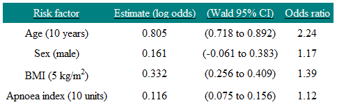
The coefficient associated with the dummy variable Sex is 0.161, so the odds of having hypertension for a man are e0.161 = 1.17 times that of a woman in this study. On the odds ratio scale the 95% confidence interval is e-0.061 to e0.383 = 0.94 to 1.47. Note that this includes one (as we would expect since the confidence interval for the regression coefficient includes zero) and so we cannot say that sex is a significant predictor of hypertension in this study. We interpret the age coefficient by saying that, if we had two people of the same sex, and given that their BMI and apnoea index were also the same, but one subject was 10 years older than the other, then we would predict that the older subject would be 2.24 times more likely to have hypertension. The reason for the choice of 10 years is because that is how age was scaled. Note that factors that are additive on the log scale are multiplicative on the odds scale. Thus a man who is ten years older than a woman is predicted to be 2.24×1.17=2.62 times more likely to have hypertension. Thus the model assumes that age and sex act independently on hypertension, and so the risks multiply.
Life Tables
Life tables (or actuarial tables) show survival patterns for groups of individuals. Specifically, they given the probability that a person in a particular age group will die before reaching the next age group. The two types of life table are:
1. Cohort life tables
These show the probability of death at each age group in a described group of individuals that has been followed over time. Cohort life tables are frequently used for survival analyses.
2. Period life tables
These give the current probability of death in given population at different ages. Period life tables are often used in demography.
To construct a cohort life table, in each time interval the following data are required: the number of people alive at the beginning of the time interval; the number of deaths occurring within the time interval; and the number of censored individuals (e.g. lost to follow-up). If we assume that on average censoring occurs at the mid-point of the time interval, the number of people at risk in any given time interval is given by the number alive at the start minus half of the number of those censored. The risk of death (and, hence, the risk of survival) can then be calculated from the number of deaths occurring during this interval.
Comparison of Survival Rates and Cox Regression
This sections covers:
- Kaplan-Meier Survival curves
- Log-rank test
- Cox regression
Survival data are times from a particular point to either an event or a censoring point. They often refer to actual survival, such as the time from diagnosis of a disease to death, but can refer to any time-dependent phenomenon, such as time in hospital until discharge, or time until a disease recurs. The latter is often termed disease-free survival. A censored observation is one where the event in question (such as death or discharge from hospital) has not happened, and all we know is that the length of time the subject has been in the study. Censored observations occur in two main ways:
1. Before the study completes, a subject may withdraw, or be lost to follow-up.
2. On completion of the study, subjects who have not yet experienced an event.
An important assumption in survival analysis is that the censoring is uninformative. What this means is that the probability of being censored is unrelated to the probability of having an event. For example, if terminally ill people are transferred to a hospice, and where they are then lost to follow-up, this would be informative censoring.
The best way to display survival data is a Kaplan-Meier survival curve. This has the probability of survival on the vertical axis, and time on the horizontal axis. Every time an event occurs, the survival curve is re-calculated by first dividing the number of events that have occurred by the number of people remaining at risk at the time. This value is then used to calculate the probability of survival. An actuarial survival curve, in contrast, calculates survival at fixed points of time, such as annually.
A risk is the probability of an event happening over a period of time. Imagine, however, that the risk varies over time. A hazard is the risk estimated at a particular point in time. An analogy would be to measure the speed of a vehicle by finding how far it travels over a fixed period of time. This would give the average speed, which is equivalent to how the risk is measured. The speed shown by the speedometer at each point in time is equivalent to the hazard. In health, think of a cohort of 100 men followed up until they are all dead. Suppose that by the age of 70, 25 had died, and in the following five years 10 die. The risk of dying between 70 and 75 is 10/100 or 0.1. The hazard of dying is conditional on a man living until he is 70, and so is 10/75=0.13.
Hazard ratios quoted in a paper can be interpreted as risk ratios or relative risks.
To compare two groups, the equivalent of the Mann-Whitney U test is the modified Wilcoxon test. An alternative is the log-rank test. These are both two-sample non-parametric tests which allow for censored observations. They differ in the weight they give to events occurring early or late in the follow-up period. Because these are tests of significance, they do not give an estimate for the magnitude of the difference between groups.
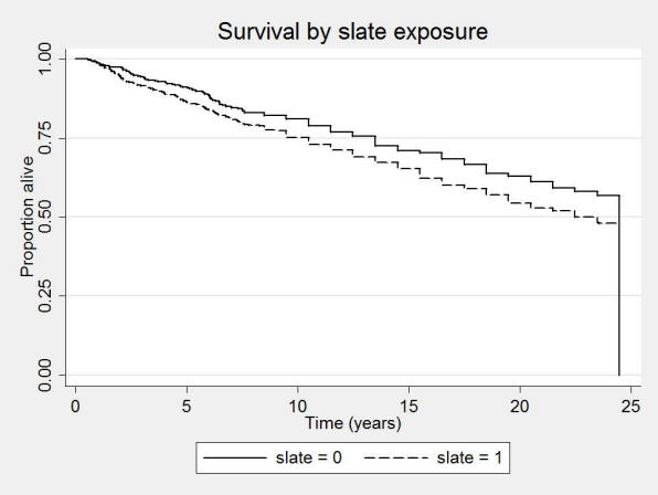
An example of a survival curve is given in Figure 1. It shows the Kaplan-Meier plot of a cohort of slate workers, and controls, over 24 years. One can see that the slate workers have a lower proportion alive compared with controls over the period. (Campbell et al 2005).
Figure 1: Kaplan-Meier survival curve
Cox Regression
The most commonly used model to analyse survival data is the Cox proportional hazards model. This models the log hazard ratio against a linear predictor of explanatory variables. Similar to other multiple regression techniques, it allows for multiple exposure variables, allowing adjustment for confounding. It is a semi-parametric model, which means that there is no requirement to parameterise the underlying survival distribution, but that the explanatory variables are included in a parametric model. The assumption of proportional hazards means that, in the two group case, the hazard in one group remains proportional to the hazard in the other group over the follow-up time, or equivalently that the relative hazard remains constant.
A parametric survival model is the Weibull model. Commonly this gives similar answer to the Cox model.
A Cox regression of the slate workers study is given in the Table 2.
Table 2: Cox regression of all-cause mortality in those under 75 years at first survey.
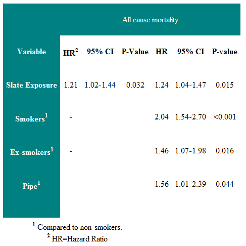
One can see that there is a 24% increased risk of death over the follow-up period in those exposed to slate dust. The right half of the table shows the regression coefficients when smoking history is included in the analysis. It can be seen that the risk of slate dust is unaffected by smoking history.
The main assumption is that this risk is constant over the follow-up period (the proportional hazard assumption).
References
- http://bmj.bmjjournals.com/cgi/content/full/317/7172/1572
- http://bmj.bmjjournals.com/cgi/content/full/328/7447/1073
- Campbell MJ. Statistics at Square Two. Chapter 4. 2nd Ed. Blackwell: BMJ Books, 2006.
- Campbell MJ, Hodges NG, Thomas HF, Paul A, Williams JG .A 24 year cohort study of mortality in slate workers in North Wales. J Occupational Medicine 2005, 55,
448-453. - Campbell MJ, Machin D and Walters SJ. (2007) Medical Statistics : A Textbook for the Health Sciences. (4th Ed) 331pp. Chichester , John Wiley & Sons Ltd
© MJ Campbell 2016, S Shantikumar 2016