Numerators, denominators and populations at risk

PLEASE NOTE:

We are currently in the process of updating this chapter and we appreciate  your patience whilst this is being completed.

 

Commonly Used Measures in Epidemiology

A principal role of epidemiology is to describe and explain differences in the distribution of disease or other health outcomes of interest between populations.

Examples of health outcomes measured in epidemiological studies include:

• Morbidity
• Mortality
• Infectious disease incidence
• Birth defects
• Disability
• Injuries
• Vaccine efficacy
• Utilisation of hospital services

Measures of disease frequency are used to describe how common an illness (or other health event) is with reference to the size of the population (the population at risk) and a measure of time.

 

Key concepts

The text below describes how to calculate the different measures of disease frequency. The following key terms are used:

 

Numerator	- The upper part of a fraction - The feature which has been counted    e.g. no. of people who have developed the disease of interest
Denominator	- The lower part of a fraction, used to calculate a rate or ratio - The population from which the numerator was derived    e.g. total no. of people in the population at risk

 

Any denominators used should be reflective of the population who could have been included in the numerator had they developed the condition of interest. This is the population at risk, and is often taken as the number of people who are disease-free at the start of data collection. If individuals who could not develop the condition of interest were included in the denominator, this would result in an underestimation of calculated rates.

There are two main measures of disease frequency:

 

Prevalence	Measures existing cases of disease and is expressed as a proportion
Incidence	Measures new cases of disease and is expressed in person-time units

 

 

1. Prevalence

Point prevalence measures the proportion of existing people with a disease in a defined population at a single point in time.

Example:

Of 10,000 female residents in town A on January 1^st 2016, 1,000 have hypertension.

The prevalence of hypertension among women in town A on this date is calculated as:

          1,000/10,000 = 0.1 or 10%

The point in time that point prevalence refers to should always be clearly stated. Prevalence is a proportion, so has no units.

Period prevalence is the number of individuals identified as cases during a specified period of time, divided by the total number of people in that population.

Prevalence is a useful measure to quantify the burden of disease in a population at a given point in time. This is of particular use when planning health services. However, prevalence is not a useful measure for establishing the determinants of disease in a population.

 

2. Incidence

Prevalence measures the frequency of existing cases of disease in a population. In contrast, incidence is a measure of the number of new cases of a disease (or another health outcome) that develop in a population of individuals at risk, during a specified time period.

There are two main measures of incidence:

 

Risk  (or cumulative incidence)	Is related to the population at risk at the beginning of the study period
Incidence   (or incidence rate)	Is related to a more precise measure of the population at risk during the study period and is measured in person time units

 

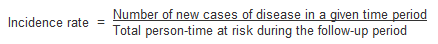
Risk

This is also known as cumulative incidence because it refers to the occurrence of risk events, such as disease or death, in a group studied over time.¹ It is the proportion of individuals in a population initially free of disease who develop the disease within a specified time interval. Incidence risk is expressed as a percentage (or, if small, as “per 1000 persons”).

Remember that the denominator is the total number of people who were free of disease at the start of the study period (the population at risk). The cumulative incidence assumes that the entire population at risk at the beginning of the study period has been followed for the specified time period for the development of the outcome under investigation. This is called a closed population.

However, in reality in a cohort study, for example, participants are followed up for a long period of time and the population will change as people enter and leave. This is called a dynamic population. Some may develop the outcome of interest, or be lost during follow-up, for a variety of other reasons:

• Refusal to continue to participate in the study
• Migration
• Death

In addition, new participants may enter the study after it starts.

 

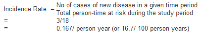
Incidence Rate

Incidence rates also measure the frequency of new cases of disease in a population, but take into account the sum of the time that each participant remained under observation and at risk of developing the outcome under investigation. This measurement also seeks to account for varying time periods of follow up, which may occur for the reasons outlined above.

 

Time at Risk

In a dynamic population, individuals in the group may have been at risk for different lengths of time, so instead of counting the total number of individuals in the population at the start of the study, the time each individual spends in the study before developing the outcome of interest needs to be calculated.

The denominator in an incidence rate is the sum of each individual's time at risk (i.e. the length of time they were followed up in the study). It is commonly expressed as person years at risk.

The incidence rate is the rate of contracting the disease among those still at risk. When a study subject develops the disease, dies or leaves the study, they are no longer at risk and will no longer contribute person-time units at risk. For example, Figure 2 illustrates the calculation of person-time units (years) at risk of a hypothetical population of 5 individuals in a 5 year cohort study.
 

Figure 1. Person-time (years) at risk for 5 individuals in a hypothetical cohort study between 2010-2014.

Year	2010	2011	2012	2013	2014	Years at risk
Person
1	-----------	-----------	-----------	-----------	-----------	5.0
2	-----------	-----------	-----------	-----------	-----x	4.5
3	-----------	-----------	-----------	-----x		3.5
4		-----------	-----x			1.5
5	-----------	-----------	-----------	-----L		3.5
Total	4	5	4.5	3	1.5	18
---  =  Time at risk X  = Developed disease L  = Person lost to follow up

In the above example the incidence rate for disease (X) is calculated as:

Note that for most rare diseases, risks and rates are numerically similar because the number at risk of developing the disease will approximately equal the total population at all times.

Issues in defining the population at risk:

• For any measure of disease frequency, a precise definition of the denominator is essential for accuracy and clarity.²
• The population at risk (denominator) should include all persons 'at risk of developing the outcome under investigation'. Therefore, individuals who currently have the disease under study or who are immune (e.g. due to immunisation), should be excluded from the denominator. However, this is not always possible in practice.²
• When individuals not at risk of the disease are included in the denominator (population at risk) the resultant measure of disease frequency will underestimate the true incidence of disease in the population under investigation.

 

Odds

Another method of measuring incidence is to calculate the odds of disease. Instead of using the number of individuals who are disease-free at the start of the study, odds are calculated using the number disease-free at the end of the time period.

 

The relationship between prevalence and incidence

The proportion of the population that has a disease at a point in time (prevalence) and the rate of occurrence of new disease during a period of time (incidence) are closely related.²

Prevalence depends on:

1. The incidence rate
2. The duration of disease

For example, if the incidence of a disease is low but the duration of disease (i.e. time until recovery or death) is long, the prevalence will be high relative to the incidence. An example of this would be diabetes.

Conversely, if the incidence of a disease is high and the duration of the disease is short, the prevalence will be low relative to the incidence. An example of this would be influenza.

A change in the duration of a disease, for example the development of a new treatment that prevents death but does not result in a cure, will lead to an increase in prevalence without affecting incidence. Fatal diseases, or diseases from which a rapid recovery is common, have a low prevalence, whereas diseases with a low incidence may have a high prevalence if they are incurable but rarely fatal and have a long duration.

The relationship between incidence and prevalence can be expressed as;

 P = ID

(P = Prevalence, I = Incidence Rate, D = Average duration of the disease)

 

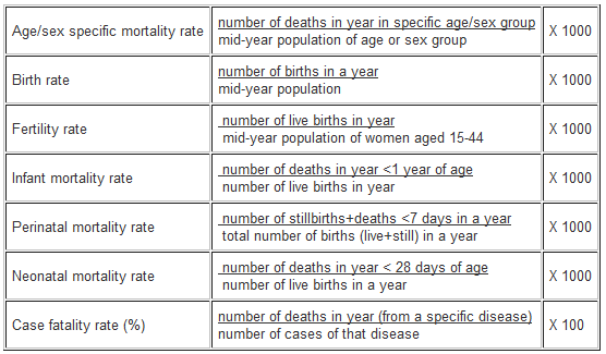
3. Other measures of disease frequency used in epidemiology
 

 

 

4. Measures of effect

Measures of effect are used in epidemiological studies to assess the strength of an association between a putative risk factor and the subsequent occurrence of disease. This is done by comparing the incidence of disease in a group of persons exposed to a potential risk factor with the incidence in a group who have not been exposed.

This comparison can be summarised by calculating either:

• The ratio of measures of disease frequency for the two groups
• The difference between the two

a) Relative measures


Relative measures reflect the increase in frequency of disease in one population (e.g. exposed) versus another (e.g. not exposed), which is treated as the baseline. They are often collectively referred to as measures of relative risk. 

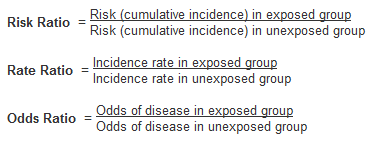
The relative risk is a measure of the strength of an association between an exposure and disease, and can be used to assess whether an observed association is likely to be causal.² The most commonly used measure of effect is the ratio of incidence rates

Rate (or risk) in exposed
Rate (or risk) in unexposed

There are three main measures of effect:

 

Risk ratios and odds ratios can be calculated using information from 2x2 contingency tables of the form:

	Outcome          No Outcome	Total
Exposure No Exposure	a               b c               d	a+b c+d
Total	a+c               b+d	a+b+c+d

 

 

 

For example, say a study randomised people with diabetes to either receive either a new hypoglycaemic drug or placebo, and looked at the proportion developing chronic kidney disease (CKD) at 5 years. Of the 100 individuals in each group, 8 on the new treatment developed CKD compared to 20 on the placebo. This information can be summarised in the following 2x2 table:

	CKD       No CKD	Total
New Drug Placebo	8               92 20             80	100 100
Total	28             172	200

 

Using this information, and the standard form of the 2x2 table above, we can calculate the risk ratio and odds ratio as follows:

 

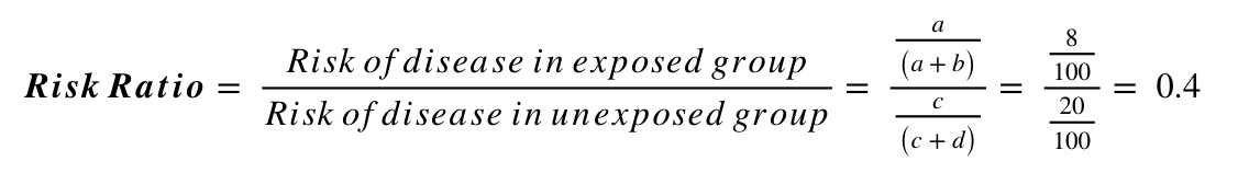
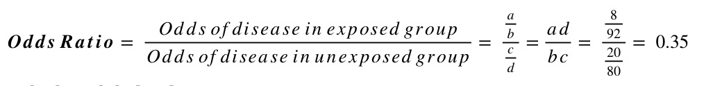
Interpreting relative risk (RR)

Measures of effect such as the risk ratio provide assessments of aetiological strength, or the strength of association between a putative risk factor and an outcome.¹

A relative risk of 1 indicates that the incidence of disease in the exposed and unexposed groups is identical and that there is no association observed between the disease and risk factor/ exposure.

A relative risk > 1 occurs when the risk of disease is greater among those exposed and indicates a positive association, or an increased risk among those exposed to the risk factor compared with those unexposed.

A relative risk < 1 occurs when the risk of disease is lower in those exposed compared to those unexposed and indicates a negative association.

Note: Rate ratios and risk ratios tend to be numerically similar for rare diseases.

 

b) Absolute measures 

Relative measures help evaluate how strongly an exposure is associated with a particular disease, but they do not give an indication of the impact of the exposure in the population. This is important for public health prevention measures.¹

Absolute measures indicate exactly what impact a disease will have on a population, in terms of numbers or proportions affected by being exposed.

For example, a study finds that having several CT head scans in childhood results in a three-fold increase of your risk of developing brain cancer as an adult. This sounds like a large increase, but because the absolute risk increase would be small (say, an increase of 0.5 cases per 10,000 children), the increased risk means one additional case of brain cancer per 20,000 children scanned.
 

Attributable Risk (Risk Difference)

The attributable risk (AR) is a measure of association that provides information about the absolute effect of the exposure or excess risk of disease in those exposed compared with the unexposed, assuming the risk is causal.² It tells us exactly how many more people are affected in the exposed group, than in the unexposed.

The risk or rate difference estimates the excess risk caused by exposure in the exposed group.

 

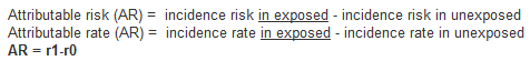
For example, in a cohort study the AR is calculated as the difference of incidence risks or incidence rates (depending on the study design used) and whether the person-time at risk is known.

An AR, assuming it is greater than zero, thus indicates the number of cases of the disease among the exposed that can be attributed to the exposure or the number of disease among the exposed that could be eliminated if the exposure were eliminated. The AR is a useful measure of the public health impact of an exposure in a population.²

 

Attributable Risk Percentage


AR may also be expressed as the proportion of disease cases in the exposed group attributable to the exposure (i.e. the proportion of additional cases in the exposed group). This is also known as the aetiologic fraction or attributable fraction. It is calculated as follows:

 

 

5. Measures of Population Impact

Measures of effect, such as relative risk, estimate the strength of an observed association between a risk factor and a disease. Attributable risk measures the extra risk or rate that is present in the exposed group compared to the unexposed group.

In contrast, measures of population impact estimate the expected impact (i.e. extra disease) in a population that can be attributed to the exposure. Again it is useful for public health purposes if we can estimate the excess disease in a population that is due to a particular risk factor.

Measures of population impact:

• Estimate how much of the disease in the population is caused by the risk factor
• Estimate the expected impact on a population of removing or changing the distribution of risk factors in that population
• Compare the population and unexposed while measures of effect compare the exposed and unexposed
• Assume that the association between disease and the risk factor are causal

There are two main measures of population impact: the population attributable risk, and the population attributable risk fraction.

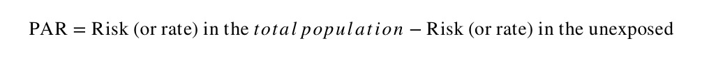
a) Population attributable risk/rate

The population attributable risk (PAR) is a similar measure to the attributable risk (or risk difference), but is concerned with the rate in the total study population (exposed + unexposed) compared with the rate in the exposed group.

The population attributable risk (PAR) estimates the excess rate of disease in the total study population that is attributable to the exposure. It provides a measure of the public health impact of the exposure in population, again assuming that the association is causal.

The PAR is the absolute difference between the risk (or rate) in the whole population and the risk (or rate) in the unexposed group, as follows:

 

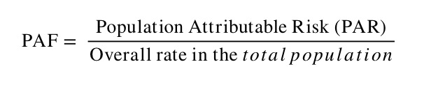
b) Population attributable risk fraction

The population attributable risk fraction (PAF) is the proportion of all cases in the whole study population (exposed and unexposed) that may be attributed to the exposure, as follows:

 

Issues in the calculation of measures of impact:

• The calculation of PAF assumes that all of the association between the risk factor and disease is causal.
• PAR varies according to how common an exposure to the risk factor is in the population.

 

6. Standardisation

A principal role of epidemiology is to compare the incidence of disease or mortality between two or more populations. However, the comparison of crude mortality or morbidity rates is often misleading because the populations being compared may differ significantly with respect to certain underlying characteristics, such as age or sex, which can affect the overall rate of morbidity or mortality.²

For example, age is an important determinant of mortality. An older population will have a higher overall mortality rate when compared to a younger population. As a result, variations in age complicate any comparison between two or more populations that have different age structures.

To understand how a comparison of crude rates can be affected by differing population distributions, it should be recognised that a crude overall rate is simply a weighted average of the individual category specific rates, with the weights being the proportion of the population in each category.² So, where a locality has a large elderly population, the older age categories will carry greater weight than the younger age categories, giving the impression that the death rate in this area is unacceptably high, particularly in comparison with a youthful town (e.g. a university town).
 

Presentation of category specific rates

One method of overcoming the effects of confounding variables such as age is to simply present and compare the age-specific rates. While this stratification allows for a more comprehensive comparison of mortality or morbidity rates between two or more populations, as the number of stratum-specific rates being compared increases, the volume of data being examined may become unmanageable.

It is, therefore, more useful to combine category specific rates into a single summary rate that has been adjusted to take into account the population’s age structure or another confounding factor. This is achieved by using the methods of standardisation.
 

Methods of Standardisation

There are two methods of standardisation commonly used in epidemiological studies. They are characterised by whether the standard used is either:

• A population distribution (direct method)
• A set of specific rates (indirect method)

Both direct and indirect standardisation involves calculating the number of expected events (e.g. deaths) and then comparing this to the number of observed events.

Age is a factor that is frequently adjusted for in epidemiological investigations, particularly in comparative mortality studies, since the age structure of a population will greatly affect the populations overall mortality. To illustrate the methods of both direct and indirect standardisation the age specific mortality rates for two hypothetical populations are compared below.
 

a) Direct standardisation

Figure 2 presents crude mortality data for two hypothetical populations (countries A and B).

The overall crude mortality rate is higher for country A (10.5 deaths / 1,000 person years) compared with country B (7 deaths / 1,000 person years), despite the age-specific mortality rates being higher among all age groups in country B.
 

Figure 2: Crude mortality rates stratified by age for two hypothetical populations.
 

 

The reason for the differences is that these two populations have markedly different age-structures. Country A has a much older population than country B. For example 18% of the population in country A are aged over 60 years compared with just 5.5% of the population in country B.

In the direct method of standardisation, 'age-adjusted rates' are derived by applying the category-specific mortality rates of each population to a single standard population (Figure 3). This produces age-standardised mortality rates that these countries would have if they had the same age distribution as the standard population.

Note that the 'standard population' used may be the distribution of one of the populations being compared or may be an outside standard population such as the European Standard Population or the WHO’s World Standard Population.
 

Figure 3: Number of people in a hypothetical standard population
 

0-29	100,000
30-59	65,000
60+	20,000
Total	185,000

 

The steps involved in direct standardisation are as follows (and illustrated in Figure 4):

1. Identify a standard population for which relevant stratum-specific data are available
    
2. Calculate the number of stratum-specific expected deaths, as follows. For each age stratum of each population being compared, multiply the age-specific mortality rate by the size of the standard population for that stratum. This essentially gives you the number of deaths one would expect in the standard population if it had the same mortality rates as your study population.
    

                  Number of expected deaths in stratum x
                                              =  observed mortality rate in stratum x
                                              X size of standard population in corresponding stratum

3. Calculate the total number of expected deaths by summing all the values from the stratum-specific calculations, above. This gives the total number of deaths that would be expected in the standard population if it had the same mortality rate as your study population.
    
4. Calculate the age-standardised rate by dividing the total number of expected deaths by the total standard population size.

 

Figure 4: Direct method of standardisation - calculation of the number of expected deaths for countries A and B applied to a standard population.

 

	Country A	Country B
Age stratum	Expected deaths	Expected deaths
0-29	0.0012 x 100,000 = 120	0.0042 x 100,000 = 420
30-59	0.0036 x 65,000 = 234	0.0055 x 65,000 = 357.5
60+	0.048 x 20,000 =  960	0.05 x 20,000 = 1,000
Total expected deaths	1,314	1,777.5
Age adjusted rate	1,314/185,000 =  7.1 per 1,000 pyrs	1,777.5/185,000 =  9.6 per 1,000 pyrs

 

The age-standardised rate provides a single summary measure for each population of interest that reflects the numbers of events that would have been expected if the populations being compared had the same age distribution.²

The ratio of the two directly standardised rates can then be calculated to provide a single summary measure that reflects the difference in mortality between the two populations. The ratio of the standardised rates is called the Comparative Mortality Ratio (CMR) and is calculated by dividing the overall age-standardised rate in, say, country B by the rate in country A. In this case example:

          Comparative Mortality Ratio = 9.6/7.1 = 1.35
 

It can thus be interpreted that, after controlling for the confounding effects of age, the mortality rate in Country B is 35% higher than in country A. While the values of the age-standardised rate do not reflect the 'true' mortality experience of countries A and B, the direct method of standardisation allows one to make a valid comparison of overall mortality between the two countries.

 

b) Indirect standardisation

The indirect method of standardisation is commonly used when age-specific rates are unavailable. For example, if we did not know the age-specific mortality rates for country B, we could not have applied direct standardisation.

In indirect standardisation, instead of taking one reference population structure as the standard and applying both sets of mortality rates to this to estimate expected events, a known set of stratum-specific rates (from either one of the populations being compared, or from a standard population) is applied to the structure of each of the populations being compared. This calculated expected rate can be compared with the overall observed rates to give a standardised morbidity/mortality ratio (SMR).

The steps involved in indirect standardisation are summarised (and illustrated in Figure 5) as follows:

1. Identify a population with stratum-specific death rates. In this case, we will use the rates from country A as the comparator.
    
2. Calculate the expected numbers of stratum-specific expected deaths. This is done by multiplying each stratum population size by the corresponding mortality rate of the comparator population.
    
                   Number of expected deaths in stratum x
                                               =  population size in stratum x
                                               X mortality rate of standard population in corresponding stratum
    
3. Calculate the total number of expected deaths by summing the number of expected deaths in each stratum. Note that if one of the study populations is being used as the “standard” comparator population, the number of expected deaths will always equal the number of observed deaths (see country A, Figure 5). As such, it doesn’t need to be calculated from scratch.
    
4. Calculate the SMR – the ratio between the observed and expected number of deaths – as follows:

    

   

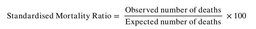
   Note that the SMR is always expressed as a percentage.

         

Figure 5: Indirect standardisation: Number of expected deaths if the population had the same age-specific mortality rates as Country A.

 

	Country A	Country B
	Expected deaths	Expected deaths
0-29	0.0012 x 6,000,000 = =7,200	0.0012 x 1,500,000 = =1,800
30-59	0.0036 x 5,500,000 =19,800	0.0036 x 550,000  = 1,980
60+	0.048 x  2,500,000 =120,000	0.048 x  120,000 =  5,760
Total expected deaths  (E)	147,000	9,540
Total observed deaths (O)	147,000	15,300

 

In this example, the expected number of deaths in Country B are calculated by multiplying the age-specific rate for Country A by the population of Country B in the corresponding age group. The sum of the age categories give the total number of deaths that would be expected in country B, if it had the same mortality experience as country A.

The SMR for country B in this example is:

         

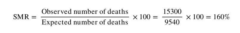
Note that by this method, the comparator population (in this case country A) has, by definition, an SMR of 100. The number of observed deaths in Country B is therefore 60% higher than what we would expect if Country B had the same mortality experience as Country A.

Issues in the use of standardisation:

• Standardised rates are used for the comparison of two or more populations; they represent a weighted average of the age-specific rates taken from a 'standard population' and are not actual rates.
• The direct method of standardisation requires that the age-specific rates for all populations being studied are available and that a standard population is defined.
• The indirect method of standardisation requires the total number of cases (e.g. number of deaths).
• The ratio of two directly standardised rates is called the Comparative Incidence Ratio or Comparative Mortality Ratio.
• The ratio of two indirectly standardised rates is called the Standardised Incidence Ratio or the Standardised Mortality Ratio.
• Indirect standardisation is more appropriate for use in studies with small numbers or when the rates are unstable.
• As the choice of a standard population will affect the comparison between populations, it should always be stated clearly which standard population has been applied.
• Standardisation may be used to adjust for the effects of a variety of confounding factors including age, sex, race or socio-economic status.

 

References

1. Carneiro I, Howard N. Introduction to Epidemiology. Open University Press, 2011.
2. Hennekens CH, Buring JE. Epidemiology in Medicine, Lippincott Williams & Wilkins, 1987.

 

 

           © Helen Barratt, Maria Kirwan 2009, Saran Shantikumar 2018